Read lsd-slam: large scale direct monolithic slam

Abstract

We propose a direct ( No features ) Monocular SLAM Algorithm , Compared with the most advanced direct method at present , This algorithm allows the construction of large-scale and consistent environment maps . A high-precision pose estimation method based on direct image alignment is adopted , At the same time, we use the position and attitude map of the key frame and the corresponding semi dense depth map , Real time reconstruction of 3D environment . This is obtained by filtering the small baseline binocular camera . The analytical representation of the scale shift allows the method to be applied to challenging sequences , Including those sequences with large scale changes in the scene . There are two innovations in this paper ：(1) stay $\mathfrak{s}\mathfrak{i}\mathfrak{m}(3)$ A new direct trace method running on , Thus the scale shift can be detected clearly ;(2) An elegant probabilistic solution , The depth value with noise is included in the tracking . The resulting direct monocular SLAM The system is in CPU Run in real time .

1 Introduce

Real time monocular simultaneous positioning and mapping (SLAM) And 3D reconstruction have become more and more popular research topics . Two main reasons are ：(1) Their applications in the field of Robotics , Especially in drones (UAV) Navigation applications ;(2) Augmented reality and virtual reality applications are slowly entering the mass market .

Monocular SLAM One of the main benefits of , And one of the biggest challenges , Is its inherent scale ambiguity . The scale of the real world cannot be observed , And will drift over time , This is one of the main sources of error . Its advantage is that it can seamlessly switch between environments of different sizes , Such as indoor desk environment and large-scale outdoor environment . On the other hand , Sensor with scale , Such as depth camera or binocular camera , The range of reliable measurements available is limited , Therefore, this flexibility cannot be provided .

1.1 Related work

A Feature-based approach

Feature-based approach ( Including filter based and key frame based ) The basic idea of is to put the whole problem , That is to estimate the geometric information from the image , Break down into two consecutive steps . First , Extract a set of feature observations from the image . secondly , The position of the camera and the geometry of the scene are calculated as a function of these feature observations .

Although this decoupling simplifies the whole problem , But it also has an important limitation . Only information that conforms to the feature type can be used . especially , When using keys , Contains information about straight or curved edges , Especially in the artificial environment, it forms a large part of the image , Will be discarded . In the past, there have been several methods to compensate for this defect by including edge based or even region based features . However , Because the estimation of high-dimensional feature space is tedious , It is rarely used in practical applications . In order to obtain dense reconstruction , Using multi view geometry, the dense map is reconstructed continuously by using the estimated camera pose .

B Direct method

Direct vision odometer (VO) Method to bypass this limitation , Directly optimize the gray level of the image to obtain geometry , This method can use all the information in the image . In addition to higher accuracy and robustness , Especially in an environment with few key points , This method can provide more information about the environment Geometry , This is very valuable for robotics or augmented reality applications .

although RGB-D Direct image alignment algorithms for cameras or binocular sensors have been well established , But it is not until recently that monocular direct VO Algorithm . In the literature [20,21,24] in , Accurate and completely dense depth maps are calculated using variational formulas , But the calculation of this method is very large , Need the most advanced GPU Run in real time . In the literature [9] in , A semi dense depth filtering formula is proposed , It greatly reduces the computational complexity , This method allows you to CPU Even running in real time on modern smartphones . By combining direct tracking with keys , The literature [10] The high frame rate real-time operation is realized on the embedded platform . However , All these methods are pure visual odometers , They only track the motion of the camera locally , Does not establish a consistent 、 Global and environment map with loopback .

C Pose optimization

This is a famous SLAM technology , For building a consistent global map . The world is represented by several keyframes connected by pose constraints , You can use a common graph optimization framework ( Such as g2o) To optimize .

In the literature [14] in , This paper presents a method based on pose graph RGB-D SLAM Method , This method introduces geometric errors , Allows tracking in scenes with fewer textures . To solve the problem of monocular SLAM Scale drift in , The literature [23] A key point based monocular SLAM System , The system expresses the camera pose as 3D Similarity transformation , Instead of rigid body motion .

1.2 Contribution and outline

We propose a large-scale direct monocular SLAM(LSD-SLAM) Method , This method can not only track the motion of the camera locally , A consistent large-scale environmental map can also be established ( See the picture 1 Sum graph 2). This method uses direct image alignment , Combined with the literature [9] Filter based semi dense depth map estimation is first proposed in . The global map is represented in the form of a pose diagram , Keyframes as vertices ,3D Similar transformation as edge , Elegantly integrated into the scale of the environment , It also allows the detection and correction of cumulative drift . The method in CPU Run in real time , Even run as a odometer on modern smartphones . The main contributions of this paper are as follows .(1) A monocular for large-scale direct SLAM Framework , In particular, a new scale aware image alignment algorithm , The similarity transformation between two key frames can be estimated directly $\xi \in \mathfrak{s}\mathfrak{i}\mathfrak{m}(3)$.(2) The probability consistently incorporates the uncertainty of the estimated depth into the tracking .

chart 1 LSD-SLAM：LSD-SLAM Generate a consistent global map , Use direct image alignment and probabilistic semi dense depth map instead of key points . Top ： Cumulative point cloud of all keyframes of the medium trajectory generated in real time ( From a hand-held monocular camera ). Bottom ： The key frame of semi dense inverse depth map with color coding . See supplementary video .

 

chart 2 In addition to accurate and semi dense 3D reconstruction ,LSD-SLAM The associated uncertainty can also be estimated . From left to right ： Limit the cumulative point cloud with different maximum variances . Notice that the reconstruction becomes significantly denser , But it also contains more noise .

 

2 Preliminary preparation (preliminaries)

In this chapter , We briefly summarize the relevant mathematical concepts and symbols . Specially , We use lie algebra to express the position and posture ( The first 2.1 section ), The weighted least squares of direct image alignment on the Lee flow is derived ( The first 2.2 section ), It also briefly introduces the propagation of uncertainty ( The first 2.3 section ).

Symbol . We use bold capital letters ($R\text{R}R$) According to matrix , Use bold lowercase letters to represent vectors ($\xi \text{ξ}\xi$). The order of the matrix $n$ Line record $[\cdot {]}_n$. The image is recorded as $I:\Omega \to \mathbb{R}$, among $\Omega \subset {\mathbb{R}}^2$ Is the normalized pixel coordinates ,$\mathbb{R}$ Represents a one-dimensional real number . Pixel level inverse depth map is marked as $D:\Omega \to {\mathbb{R}}^{+}$. The pixel level inverse depth variance graph is marked as $V:\Omega \to {\mathbb{R}}^{+}$. In the whole article , We use $d$ To indicate the depth of the road marking $z$ Reciprocal , namely $d=z^{-1}$.

2.1 3D Rigid body transformation and similarity transformation

3D Rigid body transformation . 3D rigid body transformation $G\text{G}G\in \mathrm{S}\mathrm{E}(3)$ Represents the rotation and translation of three dimensions , Write it down as
$$G\text{G}G=\left(\begin{array}{cc}R\text{R}R& t\text{t}t\\ 0\text{0}0& 1\end{array}\right)R\text{R}R\in \mathrm{S}\mathrm{O}(3),t\text{t}t\in {\mathbb{R}}^3\text{\hspace{1em}(1)}$$
In the process of optimization , Need a minimum representation of camera pose , It consists of the corresponding elements of the related Lie algebra $\xi \text{ξ}\xi \in \mathfrak{s}\mathfrak{e}(3)$ give . Lie algebras are transformed into Lie groups by exponential mapping , namely $G\text{G}G={\mathrm{e}\mathrm{x}\mathrm{p}}_{se(3)}(\xi \text{ξ}\xi )$. The inverse transformation of the mapping is $\xi \text{ξ}\xi ={\mathrm{l}\mathrm{o}\mathrm{g}}_{SE(3)}(G\text{G}G)$. Besides , We use $\mathfrak{s}\mathfrak{e}(3)$ To represent the pose , Write vectors directly $\xi \text{ξ}\xi \in {\mathbb{R}}^6$. From the coordinate system $i$ Move a point to the coordinate system $j$ The transformation of is recorded as ${\xi \text{ξ}\xi }_{ji}$. For convenience , We will connect the pose and pose operators $\circ :\mathfrak{s}\mathfrak{e}(3)\times \mathfrak{s}\mathfrak{e}(3)\to \mathfrak{s}\mathfrak{e}(3)$ Defined as ,
$${\xi \text{ξ}\xi }_{ki}:={\xi \text{ξ}\xi }_{kj}\circ {\xi \text{ξ}\xi }_{ji}:={\mathrm{l}\mathrm{o}\mathrm{g}}_{SE(3)}({\mathrm{e}\mathrm{x}\mathrm{p}}_{se(3)}({\xi \text{ξ}\xi }_{kj})\cdot {\mathrm{e}\mathrm{x}\mathrm{p}}_{se(3)}({\xi \text{ξ}\xi }_{ji}))\text{\hspace{1em}(2)}$$
further , We define the three-dimensional projection warp function $\omega$, It takes a point in the image $p\text{p}p$ And its inverse depth $d$ adopt $\xi \text{ξ}\xi$ To the camera coordinate system ,
$$\omega (p\text{p}p,d,\xi ):=\left(\begin{array}{c}{x}^{\prime }/z^{\prime }\\ y^{\prime }/z^{\prime }\\ 1/z^{\prime }\end{array}\right)with\left(\begin{array}{c}{x}^{\prime }\\ y^{\prime }\\ z^{\prime }\\ 1\end{array}\right)={\mathrm{e}\mathrm{x}\mathrm{p}}_{se(3)}(\xi \text{ξ}\xi )\left(\begin{array}{c}{p\text{p}p}_x/d\\ {p\text{p}p}_y/d\\ 1/d\\ 1\end{array}\right)\text{\hspace{1em}(3)}$$

3D Similarity transformation . A three-dimensional similarity transformation $S\text{S}S\in Sim(3)$ Including rotation 、 Zoom and pan .
$$S\text{S}S=\left(\begin{array}{cc}sR\text{R}R& t\text{t}t\\ 0\text{0}0& 1\end{array}\right)withR\text{R}R\in SO(3),t\text{t}t\in {\mathbb{R}}^{3}ands\in {\mathbb{R}}^{+}\text{\hspace{1em}(4)}$$
For rigid body transformations , The minimal representation is given by the related Lie algebra $\xi \text{ξ}\xi \in \mathfrak{s}\mathfrak{i}\mathfrak{m}(3)$ Given , Now it has an extra degree of freedom , namely $\xi \text{ξ}\xi \in {\mathbb{R}}^7$. Exponential mapping and logarithmic mapping , Pose connection (concatenation) And projection warp Functions can be similarly defined as $\mathfrak{s}\mathfrak{e}(3)$ The situation of , Further details can be found in the literature [23].

2.2 Weighted Gauss Newton optimization methods on Lie algebraic manifolds

The Gauss Newton method is used to minimize the photometric error of the two images ,
$$E(\xi \text{ξ}\xi )=\sum _i\underset{=:r_i^2(\xi )}{\underbrace{(I_{ref}({p\text{p}p}_i)-I(\omega ({p\text{p}p}_i,D_{ref}({p\text{p}p}_i),\xi \text{ξ}\xi )){)}^2}}\text{\hspace{1em}(5)}$$
Suppose there are independent identically distributed Gaussian residuals , The above formula gives a pair of $\xi \text{ξ}\xi$ Maximum likelihood estimation of . We use the left multiplication formula ： From the initial estimate ${\xi \text{ξ}\xi }^{(0)}$ Start , In each iteration , By solving $E$ Gauss Newton second order approximation of the minimum value to calculate the left multiplication increment $\delta {\xi \text{ξ}\xi }^{(n)}$.
$$\delta {\xi \text{ξ}\xi }^{(n)}=-({J\text{J}J}^{T}J\text{J}J{)}^{-1}{J\text{J}J}^{T}r\text{r}r({\xi \text{ξ}\xi }^{(n)})withJ\text{J}J=\frac{\partial r\text{r}r(ϵ\text{ϵ}ϵ\circ {\xi \text{ξ}\xi }^{(n)})}{\partial ϵ\text{ϵ}ϵ}{|}_{ϵ=0}\text{\hspace{1em}(6)}$$
among $J\text{J}J$ Is the stacking residual vector $r\text{r}r=(r_1,\cdots ,r_n{)}^T$ Multiply left increment $ϵ\text{ϵ}ϵ$ The derivative of ,${J\text{J}J}^{T}J\text{J}J$ Gauss Newton method $E$ The Hessian matrix approximation of . Then the new estimate is obtained by multiplying the calculated update ,
$${\xi \text{ξ}\xi }^{(n+1)}=\delta {\xi \text{ξ}\xi }^{(n)}\circ {\xi \text{ξ}\xi }^{(n)}\text{\hspace{1em}(7)}$$
In order to be robust to outliers from occlusion or reflection , Researchers have proposed different weighting schemes , Thus, an iterative reweighted least square problem is obtained . In each iteration , Calculate a weight matrix $W\text{W}W=W\text{W}W({\xi \text{ξ}\xi }^{(n)})$, Reduce the weight of larger residuals . The error function of iterative solution is ,
$$E(\xi \text{ξ}\xi )=\sum _i{w}_i(\xi \text{ξ}\xi )r_i^2(\xi \text{ξ}\xi )\text{\hspace{1em}(8)}$$
Update the calculation to ,
$$\delta {\xi \text{ξ}\xi }^{(n)}=-({J\text{J}J}^{T}W\text{W}WJ\text{J}J{)}^{-1}{J\text{J}J}^{T}W\text{W}Wr({\xi \text{ξ}\xi }^{(n)})\text{\hspace{1em}(9)}$$
Assume that the residuals are independent , Inverse of Hessian matrix of the last iteration $({J\text{J}J}^{T}WJ\text{WJ}WJ{)}^{-1}$ Is the covariance of the left multiply error ${\sum \text{∑}\sum }_{\xi }$ It is estimated that ,
$${\xi \text{ξ}\xi }^{(n)}=ϵ\text{ϵ}ϵ\circ {\xi \text{ξ}\xi }_{true}withϵ\text{ϵ}ϵ\sim \mathcal{N}(0,{\Sigma \text{Σ}\Sigma }_{\xi })\text{\hspace{1em}(10)}$$
actually , The residuals are highly correlated , therefore ${\Sigma }_{\xi }$ Just a lower bound —— But it contains valuable information about the correlation between noises in different degrees of freedom . Be careful , We follow the left multiplication convention , Equivalent results can be obtained by using the right multiplication convention . However , Estimated covariance ${\Sigma }_{\xi }$ Depending on the order of multiplication , When used in the pose graph optimization framework , This has to be taken into account . The left multiplication convention used here is consistent with the literature [23] Agreement , And for example ,g2o The default type implementation in is the right multiplication convention .

2.3 The spread of uncertainty

Uncertainty propagation is a statistical tool , Used to derive functions $f(X\text{X}X)$ The uncertainty of the output , Input by it $X\text{X}X$ The uncertainty of . hypothesis $X\text{X}X$ It's a Gaussian distribution , The covariance is ${\Sigma }_X\text{ΣX}{\Sigma }_X$, be $f(X\text{X}X)$ The covariance of can be approximated ( Use f Jacobian matrix of ${J\text{J}J}_f$) by ,
$${\Sigma \text{Σ}\Sigma }_f\approx {J\text{J}J}_f{\Sigma }_X\text{ΣX}{\Sigma }_X{J\text{J}J}_f^T\text{\hspace{1em}(11)}$$

3 Large scale direct monocular SLAM

We started with 3.1 The complete algorithm is outlined in section , And in 3.2 Section briefly introduces the representation of the global map . And then in 3.3 section ( Track new frames )、3.4 section ( Depth map estimation )、3.5 section ( Keyframe to keyframe tracking ) And finally 3.6 section ( Map optimization ) Three main components of the algorithm are described in .

3.1 Complete algorithm

The algorithm consists of tracking 、 Depth map estimation and map optimization are three main parts , Pictured 3 Shown .

chart 3 complete LSD-SLAM Description of algorithm

 

track The component keeps track of new camera images . in other words , It uses the pose of the previous frame as initialization , Estimate their rigid body pose relative to the current keyframe $\xi \text{ξ}\xi \in \mathfrak{s}\mathfrak{e}(3)$.

Depth map estimation The component uses the tracked frame to refine or replace the current key frame . Depth is achieved by pixel level filtering , Plus the literature [9] The interleaved space regularization proposed in . If the camera moves too far , A new key frame will be initialized by projection from the points in the existing near key frame .

Once a keyframe is replaced with a tracking reference , Therefore, its depth map will not be further refined (refine), It will be Map optimization Components are merged into the global map . To detect loop and scale drift , The similarity transformation from the current frame to the nearest key frame is estimated by scale perception $\xi \text{ξ}\xi \in \mathfrak{s}\mathfrak{i}\mathfrak{m}(3)$.

initialization . To guide LSD-SLAM System , Initialize the first key frame with random depth map and large variance . In the first few seconds , If the camera has enough translational motion , The algorithm will “ lock ” To a specific configuration , And converges to the correct depth configuration after several key frames are propagated . The attached video shows some examples . A more comprehensive assessment of this ability to converge without special initial guidance is beyond the scope of this article , And leave it for future work .

3.2 Map representation

The map is represented as the pose map of the key frame . Every keyframe ${\mathcal{K}}_i$ Contains camera pictures $I_i:{\Omega }_i\to \mathbb{R}$ And inverse depth map $D_i:{\Omega }_{D_i}\to {\mathbb{R}}^{+}$ And inverse depth variance $V_i:{\Omega }_{D_i}\to {\mathbb{R}}^{+}$. Be careful , The depth map and variance are defined only for a subset of pixels ${\Omega }_{D_i}\subset {\Omega }_i$, Contains all image regions near a sufficiently large gray gradient , So it is semi dense . Edges between keyframes contain similar transformations ${\xi \text{ξ}\xi }_{ji}\in \mathfrak{s}\mathfrak{i}\mathfrak{m}(3)$ Relative alignment of , And the corresponding covariance matrix ${\Sigma \text{Σ}\Sigma }_{ji}$.

3.3 Track new frames ： direct $\mathfrak{s}\mathfrak{e}(3)$ image alignment

From existing keyframes ${\mathcal{K}}_i=(I_i,D_i,V_i)$ Start , New images are calculated by minimizing variance normalized photometric errors $I_j$ The relative three-dimensional pose of ${\xi \text{ξ}\xi }_{ji}\in \mathfrak{s}\mathfrak{e}(3)$,
$$E_p({\xi \text{ξ}\xi }_{ji})=\sum _{p\in {\Omega }_{D_i}}\Vert \frac{r_p^2(p,{\xi }_{ji})}{{\sigma }_{r_p(p,{\xi }_{ji})}^2}{\Vert }_{\delta }\text{\hspace{1em}(12)}$$
$$with{r}_p(p,{\xi }_{ji}):=I_i(p)-I_j(\omega (p,D_i(p),{\xi }_{ji}))\text{\hspace{1em}(13)}$$
$${\sigma }_{r_p(p,{\xi }_{ji})}^2:=2{\sigma }_I^2+(\frac{\partial r_p(p,{\xi }_{ji})}{\partial D_i(p)}{)}^2{V}_i(p)\text{\hspace{1em}(14)}$$
among $\Vert \cdot \Vert$ yes Huber norm ,
$$||r^2|{|}_{\delta }:=\{\begin{array}{l}\frac{r^2}{2\delta }\mathrm{i}\mathrm{f}|r|\le \delta \\ \\ |r|-\frac{\delta }{2}\mathrm{o}\mathrm{t}\mathrm{h}\mathrm{e}\mathrm{r}\mathrm{w}\mathrm{i}\mathrm{s}\mathrm{e}\end{array}\text{\hspace{1em}(15)}$$
Applied to normalized residuals . The residual variance is calculated using covariance propagation , As the first 2.3 Section , And using the inverse depth variance $V_i$. further , We assume that the gray level of the image is Gaussian noise ${\sigma }_I^2$. As the first 2.2 Section , Use iterative reweighted Gauss Newton optimization to achieve minimization .

Compared with the previous direct method , The formula presented in this paper explicitly considers the varying noise in depth estimation . This is related to the direct monocular SLAM Especially relevant , The noise of different pixels varies greatly , It depends on how long they are visible . This is related to the treatment RGB-D The data method is the opposite , The uncertainty of the latter inverse depth is approximately constant . chart 4 It shows the performance of this weighting in different types of motion . Be careful , The depth information of the new image is unknown , Therefore, the scale of the new image is not determined , And in $\mathfrak{s}\mathfrak{e}$(3) Perform minimization on .

chart 4 Data normalization .(a) Reference image .(b-d) Trace the inverse variance of the image and the residuals \sigma_{r_p}^{-2}. For pure rotation , Depth noise has no effect on residual noise , So all normalization factors are the same . about z Translation in direction , Depth noise has no effect on the pixels in the center of the image , And for x Translation in direction , It only affects x The residual of the gray gradient in the direction .

 

3.4 Depth map estimation

Key frame selection . If the camera is too far from the existing map , A new keyframe will be created from the most recent tracking image . We weighted the relative distance and relative angle of the current key frame ,
$$\mathrm{d}\mathrm{i}\mathrm{s}\mathrm{t}({\xi \text{ξ}\xi }_{ji}):={\xi \text{ξ}\xi }_{ji}^{T}W\text{W}W{\xi \text{ξ}\xi }_{ji}\text{\hspace{1em}(16)}$$
among $W\text{W}W$ Is a diagonal matrix containing weights . Please note that , As described in the next section , Each key frame is scaled , The average inverse depth is 1. therefore , This threshold is relative to the current scene scale , And make sure that there is enough possibility to carry out stereoscopic comparison of small baseline .

chart 5 sim(3) Up direct key alignment .(a)-(c) Two keyframes 、 Depth and depth variance .(d)-(f) Photometric residuals 、 Depth residuals and Huber The weight , Before optimization ( Left ) And after optimization ( Right ).

 

Depth map creation . Once a new frame is selected as a key frame , Its depth map will be initialized by the projection points in the previous key frame , Then according to the literature [9] The method proposed in this paper performs a spatial regularization and outer point elimination . then , Zoom depth map , The average inverse depth is 1 . This scaling factor will be incorporated directly into $\mathfrak{s}\mathfrak{i}\mathfrak{m}$(3) Camera pose . Last , It replaces the previous key frame , And it is used to track the subsequent new frames .

Depth map refinement (refinement). Refine the current key frame by using the tracked frame that has not become a key frame . For an image area where the stereoscopic accuracy is expected to be large enough , Perform a large number of very effective small baseline stereo comparisons , Such as Literature [9] Described in . The results are merged into the existing depth map , To improve it and possibly add new pixels , This is the use of literature [9] The filtering method proposed in .

3.5 Constraint acquisition ： direct $\mathfrak{s}\mathfrak{i}\mathfrak{m}(3)$ image alignment

$\mathfrak{s}\mathfrak{i}\mathfrak{m}(3)$ Direct image alignment on . And RGB-D SLAM Or binocular SLAM comparison , Monocular SLAM In essence, the scale is fuzzy , That is, the absolute scale of the real world is unobservable . On a long track , This leads to scale drift , This is one of the main sources of error . Besides , All distances are defined by scale only , This leads to threshold based outlier culling or parameterized robust kernel ( Such as Huber) The definition is not clear . We use the inherent correlation between scene depth and tracking accuracy to solve this problem . The depth map of each created key frame is scaled , The average inverse depth is 1. In return , Edges between keyframes are estimated to be $\mathfrak{s}\mathfrak{i}\mathfrak{m}(3)$ The elements in , The scale difference between key frames is elegantly integrated , also , Especially for large loops , Allows explicit detection of accumulated scale drift .

So , We propose a new method in $\mathfrak{s}\mathfrak{i}\mathfrak{m}(3)$ Direct on 、 Scale shift aware image alignment , This method is used to align two keyframes with different scales . Except for photometric residuals $r_p$ outside , We also add depth residuals $r_d$, It penalizes the standard deviation of the inverse depth between keyframes , Allow direct estimation of the scaling transformation between them . The total error function to be minimized is ,
$$E({\xi \text{ξ}\xi }_{ji}):=\sum _{p\in {\Omega }_{D_i}}\Vert \frac{r_p^2(p\text{p}p,{\xi \text{ξ}\xi }_{ji})}{{\sigma }_{r_p(p,{\xi }_{ji})}^2}+\frac{r_d^2(p\text{p}p,{\xi \text{ξ}\xi }_{ji})}{{\sigma }_{r_d(p,{\xi }_{ji})}^2}{\Vert }_{\delta }\text{\hspace{1em}(17)}$$
Where photometric residuals $r_p^2$ And its variance ${\sigma }_{r_p}^2$ By formula (13) And the formula (14) Give respectively . The depth residual and its variance are calculated as ,
$$r_d(p\text{p}p,{\xi \text{ξ}\xi }_{ji}):=[{p\text{p}p}^{\prime }{]}_3-D_j([{p\text{p}p}^{\prime }{]}_{1,2})\text{\hspace{1em}(18)}$$
$${\sigma }_{r_d(p,{\xi }_{ji})}^2:=V_j([p\text{p}p{]}_{1,2}^{\prime })(\frac{\partial r_d(p\text{p}p,{\xi \text{ξ}\xi }_{ji})}{\partial D_j([{p\text{p}p}^{\prime }{]}_{1,2})}{)}^2+V_i(p\text{p}p)(\frac{\partial r_d(p\text{p}p,{\xi \text{ξ}\xi }_{ji})}{\partial D_i(p\text{p}p)}{)}^2\text{\hspace{1em}(19)}$$
among ${p\text{p}p}^{\prime }:={\omega }_s(p\text{p}p,D_i(p\text{p}p),{\xi \text{ξ}\xi }_{ji})$ Represents the transformed point . Please note that ,Huber The norm is applied to the sum of normalized photometric and depth residuals —— This explains the fact that , If one is an outlier , The other is usually an outlier . Be careful , about $\mathfrak{s}\mathfrak{i}\mathfrak{m}(3)$ Tracking on , Need to include depth error , Because only relying on photometric errors can not constrain the scale . Using iterative reweighting Gauss - Newton algorithm （ The first 2.2 section ） Yes $\mathfrak{s}\mathfrak{e}(3)$ Minimize direct image alignment on . In practice ,$\mathfrak{s}\mathfrak{i}\mathfrak{m}(3)$ Tracking is only computationally better than $\mathfrak{s}\mathfrak{e}(3)$ Tracking is a little more expensive , Because only a few extra calculations are required .

chart 6 Two large-scale scenarios . Each keyframe shows the camera frustum, Its size corresponds to the scale of the key frame .

 

Constraint search . Insert a new key frame in the map ${\mathcal{K}}_i$ after , Some possible loopback keyframes ${\mathcal{K}}_{j1},\cdots ,{\mathcal{K}}_{jn}$ Collected . We use the ten closest keyframes , And a large-scale loopback key frame candidate detected by the appearance based mapping algorithm . To avoid inserting the wrong loop or inserting the wrong trace loop , We execute a Back tracking inspection . For each candidate ${\mathcal{K}}_{jk}$, We track independently ${\xi \text{ξ}\xi }_{j_{k}i}$ and ${\xi \text{ξ}\xi }_{i{j}_k}$. Only if the two estimates are statistically similar , That is, if
$$e({\xi \text{ξ}\xi }_{j_{k}i},{\xi \text{ξ}\xi }_{i{j}_k}):=({\xi \text{ξ}\xi }_{j_{k}i}\circ {\xi \text{ξ}\xi }_{i{j}_k}{)}^T({\Sigma \text{Σ}\Sigma }_{j_{k}i}+{\mathrm{A}\mathrm{d}\mathrm{j}}_{j_{k}i}{\Sigma \text{Σ}\Sigma }_{i{j}_k}{\mathrm{A}\mathrm{d}\mathrm{j}}_{j_{k}i}^T{)}^{-1}({\xi \text{ξ}\xi }_{j_{k}i}\circ {\xi \text{ξ}\xi }_{i{j}_k})\text{\hspace{1em}(20)}$$
Small enough , They are added to the global map . therefore , Using the adjoint matrix ${\mathrm{A}\mathrm{d}\mathrm{j}}_{j_{k}i}$ take ${\Sigma \text{Σ}\Sigma }_{i{j}_k}$ Transform to the correct tangent space .

$\mathfrak{s}\mathfrak{i}\mathfrak{m}(3)$ The convergence radius of the trace . An important limitation of direct image alignment is the inherent non convexity of the problem , Therefore, a sufficiently accurate initialization is required . Although for the tracking of new camera frames , A good enough initialization is available （ Given by the pose of the previous frame ）, But when looking for loopback constraints , Is not the case, , Especially for large loops .

One solution to this is to use a very small number of keys to compute better initialization . Use depth values from existing inverse depth maps , This requires aligning two sets of 3D points , This can be done by Horn The closed form solution is effectively given by the method of . However , We found in practice that , Even for large loops , The convergence radius is also large enough . especially , We find that the convergence radius can be greatly increased by the following measures .

Efficient second order minimization (ESM). Although our results confirm previous work , namely ESM Does not significantly increase the accuracy of dense image alignment , But we observe that it does slightly increase the convergence radius .

From coarse to fine . Although pyramid method is usually used for direct image alignment , But what we found was that , from $20\times 15$ The very low resolution of pixels starts , Much smaller than usual , Helps to increase the radius of convergence .

For the evaluation of the performance of these measures, see 4.3 section .

3.6 Map optimization

The map consists of a set of keyframes and tracked $\mathfrak{s}\mathfrak{i}\mathfrak{m}(3)$ Constraints consist of , In the background, the pose graph optimization framework is used for continuous optimization . Minimizing the error function , According to the first 2.2 The left multiplication convention of stanzas , Defined by ,
$$E({\xi \text{ξ}\xi }_{W1}\cdots {\xi \text{ξ}\xi }_{Wn}):=\underset{({\xi }_{ji},{\Sigma }_{ji})\in \epsilon }{\Sigma }({\xi \text{ξ}\xi }_{ji}\circ {\xi \text{ξ}\xi }_{Wi}^{-1}\circ {\xi \text{ξ}\xi }_{Wj}{)}^T{\Sigma \text{Σ}\Sigma }_{ji}^{-1}({\xi \text{ξ}\xi }_{ji}\circ {\xi \text{ξ}\xi }_{Wi}^{-1}\circ {\xi \text{ξ}\xi }_{Wj})\text{\hspace{1em}(21)}$$
among $W$ Indicates the world system .

4 result

We are right. LSD-SLAM A quantitative assessment was carried out , Including the use of public data sets , And the challenging outdoor tracks recorded with a hand-held monocular camera . Some of the tracks evaluated are shown in the supplementary video .

4.1 Qualitative results of large trajectories

We tested the algorithm on several long and challenging trajectories , This includes many camera rotations 、 Large scale changes and big loops . chart 7 Shows an approximate 500m Long track , It takes time before and after finding the big loop 6 minute . chart 8 Shows a challenging track , There are great changes in scene depth , It also includes a loop .

chart 7 A loop of long and challenging outdoor tracks ( On the left is the loop back , On the right is the front of the loop ). It also shows three close ups of the generated point cloud , And a semi dense depth map of a specific key frame .

 

chart 8 Cumulative point cloud of trajectory under large-scale change , Including average reverse depth less than 20 Cm to greater than 10 View of meters . After the loop ( The upper right ), The geometry is aligned uniformly , And before that ( Top left ) Some scenes exist twice in different proportions . The bottom row shows different close ups of the scene . The proposed scale perception formula allows accurate estimation of fine details and large-scale geometry —— This flexibility is one of the main benefits of the monocular approach .

 

4.2 Quantitative assessment

We are publicly available RGB-D Evaluation on dataset LSD-SLAM. Please note that , For monocular SLAM Come on , This is a very challenging benchmark , Because it contains fast rotational motion 、 Strong motion blur and rolling shutter artifacts . We use the first depth map to start the system , And get the correct initial scale . chart 9 The absolute trajectory error is given , And compared with other methods .

chart 9 about TUM RGB-D Benchmark and results of two simulation sequences , With absolute trajectory error (RMSE) Form display of , In centimeters . about LSD-SLAM, We also show the number of keyframes created .x Indicates that tracking failed ,- Indicates that no data is available . For comparison , We give semi dense monocular VO[9]、 Monocular based on key points SLAM[15]、 direct RGB-D SLAM[14] And key based RGB-D SLAM Result [7]. Be careful ,[14] and [7] Use the depth information from the sensor , Others do not use .

 

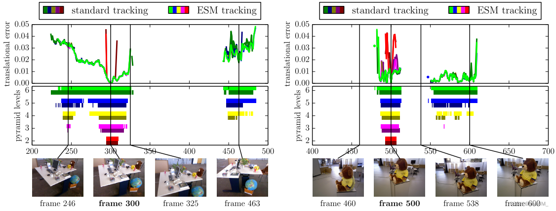
4.3 $\mathfrak{s}\mathfrak{i}\mathfrak{m}(3)$ The convergence radius of the trace

We calculate the convergence radius of two sample sequences , The result is shown in Fig. 10 Shown . Even if direct image alignment is a nonconvex optimization problem , We found that using the 3.5 Measures in section , Very large camera movements can also be tracked . It can be seen that , These methods only increase the convergence radius , It has no significant effect on tracking accuracy .

chart 10 Under different pyramid layers sim(3) The radius of convergence and the precision of , Direct image alignment , With or without ESM To minimize the ( Use light and gray to indicate ). All frames of the respective sequence are displayed on the 300 frame ( Left ) And the 500 frame ( Right ) Being tracked on , Use identity as initialization . The following figure shows the successful tracking frames ; The figure above shows the final translation error .ESM And the increase of pyramid layers obviously increases the convergence radius , But it has no significant effect on the tracking accuracy . If the tracking converges , It almost always converges to the same minimum .

 

5 Conclusion

We propose a new direct ( No features ) Monocular SLAM Algorithm , We call it LSD-SLAM, It can be CPU Run in real time . And the existing direct methods ( All are pure odometer methods ) comparison , It maintains and tracks on a global map of the environment , It contains the pose map of key frames , And the related probabilistic semi dense depth map . This approach consists mainly of two key innovations .(1) stay $\mathfrak{s}\mathfrak{i}\mathfrak{m}(3)$ Align the two keys directly on the , Explicitly merge and detect scale shifts .(2) A new probabilistic approach , The estimation of noise is added to the depth map tracking . The map is represented as a point cloud , A semi dense and highly accurate 3D reconstruction of the environment is given . Our experiments show that , This method can reliably track and plot the length over 500 M's hand-held track , Especially large-scale changes in the same sequence ( The average inverse depth is less than 20 Cm to greater than 10 rice ) And big spin , Proved its universality 、 Robustness and flexibility .

reference

A little