BM3D in popular language

Hello everyone , I meet you again , I'm your friend, Quan Jun .

---

With the release of a flagship model famous for its camera from a friend business , Its SOC in ISP5.0 The so-called SLR noise reduction algorithm BM3D It gets hot , This paper attempts to use the language as easy as possible to understand from the perspective of algorithm principle BM3D The mystery of algorithm .

---

The structure of this paper is as follows ： 1. Preface 2. Introduction to the principle of hard threshold filtering 3. Introduction to Wiener filtering principle 4.BM3D The principle is detailed 5. Principle of noise reduction in spatial domain 6. We can talk 3D Noise reduction （3DNR）

---

1. Preface Image denoising is a very important part of computer vision preprocessing , For mobile phone camera Speaking of , The quality of denoising directly affects the quality of the final image , Image denoising algorithm has experienced the traditional spatial domain denoising , Based on Fourier transform / Frequency domain filtering and noise reduction of discrete cosine transform , Partial differential equation noise reduction method based on variational method and Simulation of thermal convection , wavelet / Multiscale geometric transformation （ super-wavelets ） Multi-scale noise reduction , And now very hot based on CNN（ Deep convolution neural network ） Of AI The evolution of noise reduction and other stages . BM3D Noise reduction is an important part of Tampere University of technology in Finland （Pampere University of Technology） Of Kosadin、Alessandro、Vladimir、Karen wait forsomeone 2007 Image denoising algorithm based on traditional methods proposed in , At present, the denoising performance of this method is not AI The best effect of image denoising , Worthy of state-of-art denoising performance The title of .BM3D The basic idea comes from the observation that there are many similar repetitive structures in natural images , These similar structures are collected and aggregated by means of image block matching , Then the orthogonal transformation , Get a sparse representation of them , Make full use of sparsity and structural similarity , Filter processing ,BM3D The structure and details of the image can be fully preserved , Get a good signal-to-noise ratio .

Natural image self similar block structure

Because in BM3D In the two important steps of noise reduction algorithm, transform domain hard threshold filtering and Wiener filtering are used respectively , So I'm introducing BM3D Before , At the end of this article 2 The first part and the third part briefly introduce the basic principle of hard threshold filtering and Wiener filtering .

---

2. Introduction to the principle of hard threshold filtering Hard threshold filtering is a famous expert in signal processing and analysis Donoho 1995 The method of de-noising white noise in wavelet domain proposed in , Its basic assumption is that white noise is uniformly distributed in all scales of wavelet , But it is very small relative to the coefficient of the main signal , It can then be distinguished by a hard threshold , Coefficient less than the threshold , Set it to zero , Coefficients greater than the threshold remain unchanged , This method can achieve the purpose of signal denoising , The basic process is shown in the figure below ：

The specific process is described as follows ： （1） Transform the signal from time domain or space domain to transform domain by orthogonal transformation （2） The transform domain coefficients are filtered by hard threshold （3） The transform domain coefficients filtered by hard threshold are restored to the original time domain or space domain by orthogonal inverse transform to obtain the denoised signal Here, the hard threshold filtering is to make a simple judgment on the transform domain coefficients , If the absolute value of the coefficient is greater than the given threshold , Then keep the coefficient constant , If the absolute value of the coefficient is less than a given point threshold , Then set the coefficient to zero .

The signal here can be a one-dimensional signal , It can also be two-dimensional, three-dimensional or even high-dimensional signals , The image to be discussed in this paper is a two-dimensional signal , The orthogonal transformation here can be any orthogonal transformation designed for signal processing , Commonly used Fourier transform , Discrete cosine transform , Wavelet transform , Multiscale geometric analysis （ super-wavelets ） All are in the range of orthogonal transformation .

In order to understand the above process more vividly , Here, the hard threshold filtering processes of one-dimensional and two-dimensional signals are given respectively

close all
x = 0:0.02:3*pi;
y = 5 * cos(1 * x) + 8 * cos(3 * x)  + 7 * cos(5 * x) + 6 * cos(7 * x) + 5 * cos(10 * x);

y1 = y + 2.5 * randn(1, length(x));

freq_f1 = dct(y1);
freq_f  = dct(y);

hard_thresh = 50;

freq_signal_index = abs(freq_f1) > hard_thresh;
freq_f1_signal = freq_f1 .* freq_signal_index;

y1_hat = idct(freq_f1_signal);

y_hard = 50 * ones(1, length(x));


figure
subplot(211)
plot(x, y)
title('Original Signal')
subplot(212)
plot(x, y1)
title('Dirty Signal')

figure
subplot(511)
plot(x, y)
title('Original Signal')
subplot(512)
plot(x, y1)
title('Dirty Signal')
subplot(513)
plot(freq_f1)
title('DCT Coef of Dirty Signal')
hold on
plot(y_hard, 'r')
subplot(514)
plot(freq_f1_signal)
title('Dct Coef after Hard Shrinkage')
subplot(515)
plot(x, y1_hat)
title('Dirty Signal after Hard Shrinkage')

Copy

The red line in the figure is the given threshold , All coefficients less than the red line are changed to zero , Then the inverse transformation comes back , The dirty signal can be restored to the original signal

The signal processing process from top to bottom is shown in the figure below

As can be seen from the picture , After simple hard threshold filtering , It can filter out noise signals very well , Of course , The filtering result here is too perfect , In fact, when the noise is very loud , There will be some residual noise signals , However, the overall signal-to-noise ratio of the signal will be greatly improved .

For two-dimensional signals , Here mainly refers to digital image signal , The principle is similar , An intuitive example is also given below ,

close all
x = linspace(0, 3*pi, 128);
y = linspace(0, 3*pi, 128);
[X, Y] = meshgrid(x, y);
Z = 6 + cos(X).*cos(Y) + 8 * cos(3*X).*cos(3*Y) + 9 * cos(5*X).*cos(5*Y) + 7 * cos(7*X).*cos(7*Y);
Z1 = 10.5 * randn(128, 128) + Z;

freq_Z = dct2(Z);
freq_Z1 = dct2(Z1);

hard_thresh = 45;
freq_Z1_mask = abs(freq_Z1) > hard_thresh;
freq_Z1_hat = freq_Z1 .* freq_Z1_mask;
Z1_hat = idct2(freq_Z1_hat);


%surf(Z1)

Z_img = uint8((Z+30)/60 * 255);
Z1_img = uint8((Z1+30)/60 * 255);
Z1_hat_img = uint8((Z1_hat + 30)/60 * 255);

imshow(Z_img)
title('Original 2D Signal')
figure, imshow(Z1_img)
title('2D Signal with Noise')
figure, imshow(Z1_hat_img)
title('2D Signal After Hard Shrinkage')
figure, mesh(freq_Z)
title('2D DCT Coef of Original 2D Signal')
figure, mesh(freq_Z1)
title('2D DCT Coef of Noisy 2D Signal')
figure, mesh(freq_Z1_hat)
title('2D DCT Coef after Hard Shrinkage')

figure
subplot(151)
imshow(Z_img)
title('Original 2D Signal')
subplot(152)
imshow(Z1_img)
title('2D Signal with Noise')
subplot(153)
surf(abs(freq_Z1))
title('2D DCT Coef of Noisy 2D Signal')
subplot(154)
surf(abs(freq_Z1_hat))
title('2D DCT Coef after Hard Shrinkage')
subplot(155)
imshow(Z1_hat_img)
title('2D Signal After Hard Shrinkage')

Copy

---

3. Introduction to Wiener filtering principle Wiener filter is a statistical method to filter the stationary signal , The basic idea is to design a filter to minimize the error between the output signal and the original signal in the statistical sense , The process is shown in the figure below ：

In the process of signal acquisition or transmission , There is noise in the channel , For example, the process of taking pictures , There is thermal noise in the sensor itself , At the same time, Poisson noise also exists in the photon counting process , So our ISP The signal obtained by the processor is a noisy signal ,ISP The process of de-noising is to remove noise from CMOS RAW Restore the original photos in the data . The purpose of Wiener filter is to filter the signal y And the original signal has the smallest error in the statistical sense , That is, the mean square error is the smallest （MMSE）, It can be expressed by the following formula ： m i n E ( e 2 ) = m i n E ( ( y − s ) 2 ) min E(e^2)= min E((y-s)^2) minE(e2)=minE((y−s)2) Image signals are usually acquired and then processed , So we can use non causal Wiener filter , The expression of the system function in the frequency domain is ： H ( z ) = P x y ( z ) P s s ( z ) + P w ( z ) H(z)=\frac{P_{xy}(z)}{P_{ss}(z)+P_w(z)} H(z)=Pss​(z)+Pw​(z)Pxy​(z)​ here H ( z ) H(z) H(z) Is the frequency domain expression of Wiener filter system function , P x y ( z ) P_{xy}(z) Pxy​(z) Is the signal x And filtered signal y The power spectrum of the correlation function , P s s ( z ) P_{ss}(z) Pss​(z) Is the power spectrum of the original signal , P w ( z ) P_w(z) Pw​(z) Is the power spectrum of the noise signal . If you don't know much about statistical signal processing , Wiener filter can be regarded as a black box , After passing the black box , The signal is restored to the statistical minimum of the error with the original signal , This will achieve our goal of de-noising .

Donoho Et al. 1995 Published an article in that , White noise signal after orthogonal transformation , It is still white noise in every subspace composed of orthogonal bases , The commonly used orthogonal transformation basis function is the normalized basis function , Its power is unit power , Therefore, the power on a basis in the orthogonal transform domain is the algebraic square of the coefficient , Based on this, the method of Wiener filtering in orthogonal transform domain is point-to-point coefficient contraction to achieve the purpose of filtering , The noise level of the image can be easily estimated by statistical method , We record the variance as σ 2 \sigma^2 σ2, Then the function formula of Wiener filter system in orthogonal transform domain is given ： H = T x 2 T x 2 + σ 2 H = \frac{T_x^2}{T_x^2+\sigma^2} H=Tx2​+σ2Tx2​​ among T x T_x Tx​ Is the coefficient of the signal after orthogonal transformation , For example, Fourier transform coefficients , Discrete cosine transform coefficients , Wavelet transform coefficients, etc In the engineering , We can't get the original signal , Therefore, it is impossible to get the orthogonal transform coefficient of the original signal and put it into the Wiener filter for filtering , The simplest method is to take the noise signal as the original signal and carry out orthogonal transformation into the Wiener filtering formula to get the filtering result , But this effect is usually not ideal , The following is a set of experimental results

From the perspective of image effect , Directly take the noisy signal as the original signal and bring it into the Wiener filtering system function for Wiener filtering , The effect is not so good , from 2D-DCT The same is true in terms of coefficient . Therefore, the Wiener filter is improved , Hard threshold filtering for noisy signals , The obtained signal is brought into the Wiener filter system function as the original signal , Then Wiener filtering is applied to the noisy signal after any operation , The result is better , Here is a set of experiments ：

clear
clc
close all
x = linspace(0, 3*pi, 128);
y = linspace(0, 3*pi, 128);
[X, Y] = meshgrid(x, y);
Z = 6 + cos(X).*cos(Y) + 8 * cos(3*X).*cos(3*Y) + 9 * cos(5*X).*cos(5*Y) + 7 * cos(7*X).*cos(7*Y);
Z1 = 10.5 * randn(128, 128) + Z;

freq_Z = dct2(Z);
freq_Z1 = dct2(Z1);

sigma = 20.5^2;
hard_thresh = 35;

winer_filter_ideal =  freq_Z.^2 ./ (freq_Z.^2 + sigma);
winer_filter = freq_Z1.^2 ./ (freq_Z1.^2 + sigma);
freq_Z1_hat_ideal = winer_filter_ideal .* freq_Z1;
freq_Z1_hat = winer_filter .* freq_Z1;
Z1_hat = dct2(freq_Z1_hat);
Z1_hat_ideal = dct2(freq_Z1_hat_ideal);

freq_Z1_mask = abs(freq_Z1) > hard_thresh;
freq_Z1_hard = freq_Z1 .* freq_Z1_mask;
freq_Z1_hat_hard = freq_Z1_hard.^2 ./ (freq_Z1_hard.^2 + sigma) .* freq_Z1;
Z1_hat_hard = dct2(freq_Z1_hat_hard);


Z_img = uint8((Z+30)/60 * 255);
Z1_img = uint8((Z1+30)/60 * 255);
Z1_hat_img = uint8((Z1_hat + 30)/60 * 255);
Z1_hat_img_ideal = uint8((Z1_hat_ideal + 30)/60 * 255);
Z1_hat_img_hard = uint8((Z1_hat_hard + 30)/60 * 255);

figure, imshow(Z_img);
title('Original 2D Signal')
figure, imshow(Z1_img);
title('Noisy 2D Signal')
figure, imshow(Z1_hat_img);
title('2D Signal After Wiener Filtering')
figure, imshow(Z1_hat_img_ideal)
title('2D Signal After Hard Wiener Filtering')
figure, mesh(freq_Z);
title('2D DCT Coef of Noisy Signal')
figure, mesh(freq_Z1);
title('2D DCT Coef of Original Signal')
figure, mesh(freq_Z1_hat);
title('2D DCT Coef After Wiener Filtering')
figure, mesh(freq_Z1_hat_ideal)
title('2D DCT Coef After Hard Wiener Filtering')

figure, mesh(freq_Z1_hat_hard)
figure, imshow(Z1_hat_img_hard)

Copy

This time, we can see that the experimental results have been significantly improved , No matter from the image effect , still 2D-DCT The spectrum coefficient is the same .

Someone will ask. , Since the previous section has pointed out , Good results can be obtained directly through hard threshold filtering , Why do I do a hard threshold filter here , And then put it into the Wiener filter for Wiener filtering ？ This is because , It is difficult to find a suitable threshold to distinguish signal and noise in engineering , be prone to “ Accidental injury ” Small coefficient real signal , In Wiener filter, the system function H It can be divided into three situations ：（1） When the signal power is very small, the noise is dominant , that H It's almost zero ,H Multiply by the noisy signal coefficient , The coefficient of noisy signal is almost equal to zero , Good noise suppression ;（2） When the signal power is large, the signal is dominant , that H Almost equal to one ,H Multiply by the noisy signal coefficient , The signal is almost constant , The signal is well preserved ;（3） When the noise power is about the same as the signal power , At this time, the signal and noise account for half ,H The value of is equal to about one-half ,H Multiply by the noisy signal coefficient , The noise coefficient is approximately restored to the original signal coefficient ; Based on the analysis of the above three situations , Wiener filter can reduce the “ Accidental injury ”, It has better results than direct hard threshold filtering , In addition, Wiener filtering is a filtering method with the minimum error in the statistical sense . The introduction is over. BM3D The two filtering techniques used in the transform domain , Let's get down to business , Introduce BM3D The basic principle of .

---

4.BM3D The principle is detailed BM3D Full name Block Matching and 3D collaborative filtering, Based on block matching 3D Collaborative filtering , The central idea of the algorithm is to make full use of the abundant self similar structures in natural images to reduce image noise .

BM3D The process of noise reduction algorithm is divided into two stages , The first stage is called basic estimation filtering , The second stage is called final estimation filtering , The process is shown in the figure below ：

The first stage ： a) Block matching estimation ：i) Block matching grouping ii)3D Cooperative hard threshold filtering b) Aggregate weighted filtering The second stage ： a) Block matching estimation ：i) Block matching grouping ii)3D Cooperative Wiener filtering b) Aggregate weighted filtering

Let's follow the data flow in the process , Detailed instructions BM3D Filtering process

1) The first stage is block matching ： Search the image block similar to the given image block in the way of window drawing , If the similarity with the image is high , Then add it to the group , If the similarity is not high , Abandon , Continue to look for the next similar image block , What needs special explanation is , There is an inverse correlation between image similarity and image difference , Before the similarity comparison, a hard threshold shrinkage is performed on the image block , Remove the influence caused by high-frequency noise , The dynamic process of block matching is shown in the following figure

2) The first stage 3D Cooperative hard threshold filtering ： The image block obtained in the previous process is 3D Orthogonal transformation of , Hard threshold filtering in transform domain , And then inverse transform to the spatial domain , obtain 3D Image block filtered by cooperative hard threshold , Then put the filtered image blocks back to their original image positions

there 3D Orthogonal transform makes full use of the correlation within image blocks and the correlation between image blocks , Inside the image block composed of the first two-dimensional space in the above figure , One 2D The orthogonal transformation of the image reveals the internal correlation of the image , All image blocks pass through the first 2D After orthogonal transformation , The pixels at the corresponding positions are strung along the third dimension , In the third dimension 1D Orthogonal transformation of , This orthogonal transformation reveals the correlation between image blocks , It makes full use of the similarity of the same group of image blocks to express the coefficients , Through this first 2D Orthogonal transformation reconstruction 1D Formed by orthogonal transformation 3D Orthogonal transform hard threshold filtering , It can suppress the image noise very well , At the same time, the unique details of each image block in the group of image blocks are preserved .

3) The first stage is aggregation weighted filtering ： After the first 2) Medium 3D After collaborative filtering , Put the image block back to its original position , But when searching for similar image blocks , There is overlap of image blocks , As shown in the figure above, several image blocks in the red area , There are overlapping areas between each other , Then there will be more than one denoised result for the pixels in the overlapping area , Which one to take , The method to deal with this problem is called aggregate weighted filtering , That is, different estimated values of the same pixel are given a weight , Take the weighted average result as the final result .

4) The second stage is block matching After the first stage of basic estimation filtering, a basic estimation filtered image is obtained , Then we estimate the block matching , Get a new group , Then, the original noisy images without denoising are grouped according to the basic filtering at the same position , The original noisy images are also grouped in the same way , The specific block matching process is similar to the first stage block matching process , I won't repeat it here , It should be noted that , Here we get two block matching groups , A grouped image block comes from the filtered image after the basic estimation in the first stage , We call it a Group , The other group comes from noisy images without any processing , We call it b Group . 5) Second order 3D Cooperative Wiener filtering After getting the two packets of block matching in the second stage , We will a Group as a guide image block , As the original image polluted by noise ,b Group images are treated as images to be denoised , The two groups were tested respectively 3D Orthogonal transformation , Then, as introduced in the third part of the text , Wiener filtering , After Wiener filtering , Yes b Group progress 3D Inverse intersection transform to spatial domain image block , And put the image block of the image block back to its original position . 6) The second stage is aggregation weighted filtering The same as the first stage aggregation weighted filtering , Here to b Group of image data is filtered by aggregation weighting , obtain BM3D The end result of .

Careful analysis BM3D The two-stage filtering details of , In the first stage, the image is block matched ,3D Image obtained by collaborative filtering , Not directly contribute to the final image results , But the filtered result noise is less than the original noise , The effect of block matching is more accurate , So it can be used to guide the block matching and 3D The weight calculation of Wiener filtering system function in collaborative filtering , After obtaining the weight, the pixels that really participate in the collaborative filtering are still the original noisy images ,3D After Wiener filtering, the inverse transform returns to the spatial domain, and then the image block is weighted , Get the final de-noising result , So the real de-noising process is the second stage , The techniques involved in denoising include Wiener filtering in transform domain and linear weighting in spatial domain .

Through a simple extension , You can filter the gray image BM3D Extended to the filtering of color images C-BM3D, there C Representative color color.

thus BM3D The noise reduction algorithm is introduced .

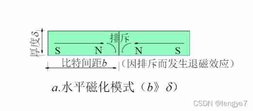
5. The principle of noise reduction in spatial domain is detailed At the end of the article , I want to say a few words , This paper introduces the reason why the weighted average between pixels in spatial domain can achieve the purpose of noise reduction （1） Weighted average in spatial domain is essentially a low-pass filter , How to allocate the weight determines the performance index of the rate filter, such as the filter band block shape （2） From the point of view of random variables , Noise signal is usually assumed to be an independent identically distributed random variable , namely ： Suppose there is n Pixels participate in the weighting , Their noise components are x ( i ) clothing from N ( 0 , σ 2 ) , i . i . d , i = 1 , 2 , ⋯   , n x(i) obey N(0,\sigma^2), i.i.d, i=1,2,\cdots,n x(i) obey N(0,σ2),i.i.d,i=1,2,⋯,n, The weight of ω 1 , ω 2 , ⋯   , ω n \omega_1,\omega_2,\cdots,\omega_n ω1​,ω2​,⋯,ωn​, And ω 1 + ω 2 + ⋯ + ω n = 1 \omega_1+\omega_2+\cdots+\omega_n=1 ω1​+ω2​+⋯+ωn​=1, that x = ω 1 x ( 1 ) + ω 2 x ( 2 ) + ⋯ + ω n x ( n ) x=\omega_1x(1)+\omega_2x(2)+\cdots+\omega_nx(n) x=ω1​x(1)+ω2​x(2)+⋯+ωn​x(n) It is easy to get from the sum of variance formula v a r ( x ) = ω 1 2 σ 2 + ω 2 2 σ 2 + ⋯ + ω n 2 σ 2 = ( ω 1 2 + ω 2 2 + ⋯ + ω n 2 ) σ 2 \begin{aligned} var(x) &=\omega_1^2\sigma^2+\omega_2^2\sigma^2+\cdots+\omega_n^2\sigma^2 \\ &=(\omega_1^2 + \omega_2^2 + \cdots + \omega_n^2)\sigma^2 \end{aligned} var(x)​=ω12​σ2+ω22​σ2+⋯+ωn2​σ2=(ω12​+ω22​+⋯+ωn2​)σ2​ It can be seen from the above formula that the noise variance becomes the original after weighting ω 1 2 + ω 2 2 + ⋯ + ω n 2 \omega_1^2+\omega_2^2+\cdots+\omega_n^2 ω12​+ω22​+⋯+ωn2​, And there are ω 1 + ω 2 + ⋯ + ω n = 1 \omega_1+\omega_2+\cdots+\omega_n=1 ω1​+ω2​+⋯+ωn​=1 constraint condition , Such an optimization problem is easy to get , In a certain ω = 1 \omega=1 ω=1 when , The others are zero , At this time, only one block or pixel is weighted , It has the largest noise variance , by σ 2 \sigma^2 σ2, It is easy to analyze by Lagrange multiplier , stay ω 1 = ω 2 = ⋯ = ω n = 1 n \omega_1=\omega_2=\cdots=\omega_n=\frac{1}{n} ω1​=ω2​=⋯=ωn​=n1​ when n Image blocks or pixels are weighted , Minimum noise variance , become 1 n σ 2 \frac{1}{n}\sigma^2 n1​σ2, By this mathematical process , When using spatial domain image denoising , It is necessary to search for similar image blocks or pixels for weighting , In this way, their weights are close to each other , The noise variance of the weighted result is the smallest , Better images .

6. We can talk 3D Noise reduction （3DNR） From the independent repeated experiment of probability theory , For example, we count the number of dice thrown as 1 What's the probability of , We can make a person throw 10000 times , Then the number of points in the statistical result is 1 The number of , Thus, the number of dice thrown is calculated as 1 Probability （ In the sense of the law of large numbers ）, Another way is to let 1000 personal , Each person throws dice ten times , Then count the points as 1 Probability ; It can be seen from the above two experiments , We want to get a lot of samples of a random event , This event can be made to adopt an experimental method , Let random events repeat N Time , Get the statistical law , You can also construct many m The same randomized experiment , Then repeat for each randomized trial N/m Time , In this way, on the whole , In general, the same random events are repeated N, The statistical law obtained is consistent with the previous conclusion . Back to image denoising , We know that the noisy image signal is the sum of a fixed image signal and a noise random variable , Then the image signal we observed is also a random variable , We want to get the real signal by weighting , So we need this random variable N Samples . Where did such samples come from , One way to do this is to N Secondary observation , This method corresponds to the fusion of multiple frames of the same exposure image we use in engineering 3D Noise reduction algorithm , This method is similar to what a person does N Repeat the experiment independently ; Another way is to find the same image block in itself , One of its implementation methods is mentioned in this article BM3D, This method is similar to N personal , Everyone did an independent repeat experiment .

---

reference

1. Kostadin Dabov, Alessandro Foi, Vladimir Kathovnik, Karen Egiazarian, “Image denoising by sparse 3D transform-domain collaborative filtering”, IEEE Transaction on Image Processing, Vol. 16, No. 8. August 2007
2. http://www.cs.tut.fi/~foi/GCF-BM3D/
3. Hu Guangshu , Digital signal processing —- theory 、 Algorithm and Implementation , The third edition ,2012

Publisher ： Full stack programmer stack length , Reprint please indicate the source ：https://javaforall.cn/133832.html Link to the original text ：https://javaforall.cn