cartographer_ fast_ correlative_ scan_ matcher_ 2D branch and bound rough matching

0. introduction

fast_correlative_scan_matcher_2d It's right real_time_correlative_scan_matcher_2d Accelerated optimization of algorithm .

The documents involved are ：

• mapping/internal/constraint/constraint_builder_2d.cc :

    /** * @brief  Perform constraint calculation of local search window ( Loop back detection for local subgraphs ) * * @param[in] submap_id submap Of id * @param[in] submap  Single submap * @param[in] node_id  Node id * @param[in] constant_data  Node data  * @param[in] initial_relative_pose  The initial value of the constraint  */
    void ConstraintBuilder2D::MaybeAddConstraint(
        const SubmapId& submap_id, const Submap2D* const submap,
        const NodeId& node_id, const TrajectoryNode::Data* const constant_data,
        const transform::Rigid2d& initial_relative_pose) {
        
      //...
      
      //  Create a new matcher for the subgraph 
      const auto* scan_matcher =
          DispatchScanMatcherConstruction(submap_id, submap->grid());
    
      //  Generate a calculation constraint task 
      auto constraint_task = absl::make_unique<common::Task>();
      constraint_task->SetWorkItem([=]() LOCKS_EXCLUDED(mutex_) {
        
        ComputeConstraint(submap_id, submap, node_id, false, /* match_full_submap */
                          constant_data, initial_relative_pose, *scan_matcher,
                          constraint);
      });
      // ...
    }
  

  /** * @brief  Compute a constraint between nodes and subgraphs ( Loop back detection ) *  Rough matching with a matcher based on branch and bound algorithm , And then use ceres Perform fine matching  * * @param[in] submap_id submap Of id * @param[in] submap  Map data  * @param[in] node_id  node id * @param[in] match_full_submap  Is it local matching or full subgraph matching  * @param[in] constant_data  Node data  * @param[in] initial_relative_pose  The initial value of the constraint  * @param[in] submap_scan_matcher  matcher  * @param[out] constraint  Calculated constraints  */
  void ConstraintBuilder2D::ComputeConstraint(
      const SubmapId& submap_id, const Submap2D* const submap,
      const NodeId& node_id, bool match_full_submap,
      const TrajectoryNode::Data* const constant_data,
      const transform::Rigid2d& initial_relative_pose,
      const SubmapScanMatcher& submap_scan_matcher,
      std::unique_ptr<ConstraintBuilder2D::Constraint>* constraint) {
        
  	// ...
    // Step:2  Use the matcher based on branch and bound algorithm for rough matching 
      if (submap_scan_matcher.fast_correlative_scan_matcher->Match(
              initial_pose, constant_data->filtered_gravity_aligned_point_cloud,
              options_.min_score(), &score, &pose_estimate)) {
        
        // We've reported a successful local match.
        CHECK_GT(score, options_.min_score());
        kConstraintsFoundMetric->Increment();
        kConstraintScoresMetric->Observe(score);
      } else {
        
        return;
      }
    // Step:3  Use ceres Perform fine matching ,  It is the function used for front-end scan matching 
    ceres::Solver::Summary unused_summary;
    ceres_scan_matcher_.Match(pose_estimate.translation(), pose_estimate,
                              constant_data->filtered_gravity_aligned_point_cloud,
                              *submap_scan_matcher.grid, &pose_estimate,
                              &unused_summary);
      //....
  

• mapping/internal/2d/scan_matching/fast_correlative_scan_matcher_2d.cc :

• mapping/internal/2d/scan_matching/real_time_correlative_scan_matcher_2d.cc :

Every step of the following is for a pair node<-->submap Prepare for constraints between subgraphs .

1. Multi resolution map construction

  //  Create a new matcher for the subgraph 
  const auto* scan_matcher =
      DispatchScanMatcherConstruction(submap_id, submap->grid());

//  Create a new matcher for each subgraph 
const ConstraintBuilder2D::SubmapScanMatcher*
ConstraintBuilder2D::DispatchScanMatcherConstruction(const SubmapId& submap_id,
                                                     const Grid2D* const grid) {
    
  CHECK(grid);
  // ...
  auto& scan_matcher_options = options_.fast_correlative_scan_matcher_options();
  auto scan_matcher_task = absl::make_unique<common::Task>();
  //  Generate a task that will initialize the matcher ,  The multi-resolution map will be calculated during initialization ,  More time-consuming 
  scan_matcher_task->SetWorkItem(
      [&submap_scan_matcher, &scan_matcher_options]() {
    
        //  Initialize the matcher ,  With the creation of multi-resolution maps 
        submap_scan_matcher.fast_correlative_scan_matcher =
            absl::make_unique<scan_matching::FastCorrelativeScanMatcher2D>(
                *submap_scan_matcher.grid, scan_matcher_options);
      });
  //...
}

stay FastCorrelativeScanMatcher2D Constructor to build multi-resolution map at the same time .

• PrecomputationGrid2D: Maps of different resolutions
• PrecomputationGridStack2D： Map storage with different resolutions

  //  The resolution increases gradually , i=0 Is the default resolution 0.05, i=6 when , width=64, That is to say 64 A lattice composes a value 
  for (int i = 0; i != options.branch_and_bound_depth(); ++i) {
    
    const int width = 1 << i;  // 2^i
    //  Construct maps of different resolutions  PrecomputationGrid2D
    precomputation_grids_.emplace_back(grid, limits, width,
                                       &reusable_intermediate_grid);
  }

offset I don't want to take a closer look at the calculation of what , There is no difficulty , Just trim it carefully , You can refer to When the front-end map grows ：

Slide the window to create a multi-resolution map ：

Actually, the grid is still there , Only the value becomes the maximum value , Some small details can be seen in the code ：

therefore , It can be concluded that the stored data is similar to the image pyramid but different （ The size of the overall picture has not changed , Multiresolution map cell The number doesn't change , Just every one cell The probability value of is equal to the maximum value of all probabilities in the large resolution , Not merged into a large grid ）, At the bottom （front） The highest resolution of is the original resolution （0.05m）：

for (int i = 0; i != options.branch_and_bound_depth(); ++i) {
    
  const int width = 1 << i;  // 2^i
  //  Construct maps of different resolutions  PrecomputationGrid2D
  precomputation_grids_.emplace_back(grid, limits, width,
                                     &reusable_intermediate_grid);
}

The final results are shown in the paper ：

2. Generate candidate frames

Most of the front is related to Front end violence matching The steps are the same , stay $\theta$ After generating candidate sets in steps , For the search window ($x,y$） It is further reduced according to the actual situation ：

  //  Reduce the size of the search window ,  Calculate the maximum moving range of each frame point cloud when the last point can be within the map range 
  search_parameters.ShrinkToFit(discrete_scans, limits_.cell_limits());

• Get the lowest resolution layer ( The grid is the thickest ) And calculate the score of each candidate solution , Sort according to the matching score from big to small , Return to the arranged candidates , This step is no different from the front end .

  const std::vector<Candidate2D> lowest_resolution_candidates =
        ComputeLowestResolutionCandidates(discrete_scans, search_parameters);
  

3. Filter the best candidate frames based on branch and bound

/** * @brief  Branch and bound search algorithm based on multi-resolution map  * * @param[in] discrete_scans  Grid coordinates of each point of multiple point clouds on the map  * @param[in] search_parameters  Search for configuration parameters  * @param[in] candidates  Candidate solution  * @param[in] candidate_depth  Search tree height  * @param[in] min_score  Minimum score of candidate points  * @return Candidate2D  Optimal solution  */
Candidate2D FastCorrelativeScanMatcher2D::BranchAndBound(
    const std::vector<DiscreteScan2D>& discrete_scans,
    const SearchParameters& search_parameters,
    const std::vector<Candidate2D>& candidates, const int candidate_depth,
    float min_score) const {
    

This article It is easy to understand the explanation of branch and bound , Carry a little ：

---

• The process of branching is the process of adding child nodes to the tree

• Delimit （ Pruning process ） Is to check the upper and lower bounds of the subproblem in the process of branching （ If the problem is to find the maximum value, set the last , The minimum is the lower bound ）, If the subproblem cannot produce a better solution than the current optimal solution , Then cut off the whole one . Until none of the subproblems can produce a better solution , The algorithm ends

• A Root node , Represents the entire solution space ω
• JKLMNOPQ Is a leaf node , Represents a specific solution
• BCDEFGHI It's an intermediate node , Represent the solution space ω Some part of the molecular space of

Specific process ：

• A m. BCDE, Sort by priority ;

• B m. FGHI, Sort by priority ;

• F m. JKLM, Sort by priority ;

• On the leaf node , Calculation JKLM The maximum value of the objective function , Write it down as best_score（ The initial value is negative infinity ）;

• Go back to the previous level G, Calculation G The value of the objective function of , And best_score Compare ：

• if best_score Still the biggest , On the other hand G Pruning , Continue to calculate H The value of the objective function of ;

• if G The objective function value of is greater than best_score, On the other hand G Branching NOPQ, Calculation NOPQ The maximum value of the objective function , And best_score Compare , to update best_score;

---

This article The reason for setting the probability value of multi-resolution map is well explained . In fact, the essence of branch and bound is depth first search plus a pruning operation ：

• 1、 Search from the root node , Search to The lowest leaf node , obtain score The maximum of , Write it down as best_score.

• 2、 Return to the previous node , Let's see if its score is greater than best_score, If it is , Continue branching （ If there is still more than at the bottom layer best_score The score of is updated best_score And record ）, If not , You can prune directly , Discard this node and all child nodes . Because the score of a node represents the upper bound of the score of its child nodes , If the upper bounds are less than best_score, It is impossible for any child node to score higher than it .

This article Examples are easy to understand :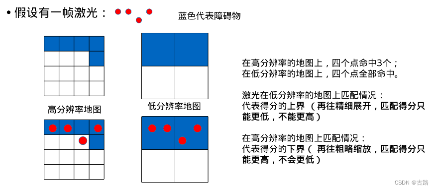

Clear thinking , So let's look at the code DFS：

In fact, the solutions are sorted , So it's faster , The solution will only be found in the left part ！

/** * @brief  Branch and bound search algorithm based on multi-resolution map  * * @param[in] discrete_scans  Grid coordinates of each point of multiple point clouds on the map  * @param[in] search_parameters  Search for configuration parameters  * @param[in] candidates  Candidate solution  * @param[in] candidate_depth  Search tree height  * @param[in] min_score  Minimum score of candidate points  * @return Candidate2D  Optimal solution  */
Candidate2D FastCorrelativeScanMatcher2D::BranchAndBound(
    const std::vector<DiscreteScan2D>& discrete_scans,
    const SearchParameters& search_parameters,
    const std::vector<Candidate2D>& candidates, const int candidate_depth,
    float min_score) const {
    

  //  This function is solved recursively 
  //  First, the conditions of recursive termination are given ,  That is, if you arrive at the 0 layer ( Whether the ),  It means that we have found a leaf node .
  //  At the same time, in each iteration process, we arrange the candidate points of the new extension in descending order 
  //  So the leaf node of the team leader is the optimal solution ,  Just go back 
  if (candidate_depth == 0) {
    
    // Return the best candidate.
    return *candidates.begin();
  }

  //  Then create a temporary candidate solution ,  And set the score to min_score
  Candidate2D best_high_resolution_candidate(0, 0, 0, search_parameters);
  best_high_resolution_candidate.score = min_score;

  //  Traverse all candidate points 
  for (const Candidate2D& candidate : candidates) {
    
    // Step:  prune   Below set threshold   perhaps   The highest score of a feasible solution lower than the upper level   The feasible solution of does not continue to branch 
    //  If the score of a candidate point is lower than the threshold ,  Then the score of the candidate solution behind will also be lower than the threshold , You can jump out of the loop 
    if (candidate.score <= min_score) {
    
      break;
    }

    //  If for The loop can continue to run ,  It indicates that the current candidate point is a better choice ,  It needs to be branched 
    std::vector<Candidate2D> higher_resolution_candidates;
    //  The search step is reduced to half of the upper level 
    const int half_width = 1 << (candidate_depth - 1);

    // Step:  m.   Yes x、y Offset to traverse ,  Find out candidate Four child node candidate solutions of 
    for (int x_offset : {
    0, half_width}) {
     //  Can only take 0 and half_width
      //  If you exceed the limit ,  Just skip. 
      if (candidate.x_index_offset + x_offset >
          search_parameters.linear_bounds[candidate.scan_index].max_x) {
    
        break;
      }
      for (int y_offset : {
    0, half_width}) {
    
        if (candidate.y_index_offset + y_offset >
            search_parameters.linear_bounds[candidate.scan_index].max_y) {
    
          break;
        }

        //  The candidates advanced in turn ,  altogether 4 individual , It can be seen that ,  The branch and bound method branches the four child nodes in the lower right corner 
        higher_resolution_candidates.emplace_back(
            candidate.scan_index, candidate.x_index_offset + x_offset,
            candidate.y_index_offset + y_offset, search_parameters);
      }
    }

    //  For the newly generated 4 Score and sort the candidate solutions ,  The same point cloud ,  Different maps  -->  To the corresponding multiresolution map 
    // depth: 7-->0  The resolution of the ： low （ Thick grid ）-->  high （ Fine lattice ）
    ScoreCandidates(precomputation_grid_stack_->Get(candidate_depth - 1),
                    discrete_scans, search_parameters,
                    &higher_resolution_candidates);

    //  Recursively call BranchAndBound For the newly generated higher_resolution_candidates To search  
    //  Continue to branch to the node with the highest score ,  Up to the bottom ,  Then return to the penultimate layer for iteration 
    //  If the highest score of the penultimate layer is not the lowest score of the previous one （ Cotyledon layer ） The score is high ,  Then skip , 
    //  Otherwise, continue to branch down and score 
 
    // Step:  Delimit  best_high_resolution_candidate.score
    //  In the future, better solutions found through recursive calls will pass std::max Function to update the known optimal solution .
    best_high_resolution_candidate = std::max(
        best_high_resolution_candidate,
        BranchAndBound(discrete_scans, search_parameters,
                       higher_resolution_candidates, candidate_depth - 1,
                       best_high_resolution_candidate.score));
  }
  return best_high_resolution_candidate;
}

Learn to think , The details will be forgotten for a long time .

4.ceres_scan_matcher_2d Fine matching

go back to mapping/internal/constraint/constraint_builder_2d.cc

/** * @brief  Compute a constraint between nodes and subgraphs ( Loop back detection ) *  Rough matching with a matcher based on branch and bound algorithm , And then use ceres Perform fine matching  * * @param[in] submap_id submap Of id * @param[in] submap  Map data  * @param[in] node_id  node id * @param[in] match_full_submap  Is it local matching or full subgraph matching  * @param[in] constant_data  Node data  * @param[in] initial_relative_pose  The initial value of the constraint  * @param[in] submap_scan_matcher  matcher  * @param[out] constraint  Calculated constraints  */
void ConstraintBuilder2D::ComputeConstraint(
    const SubmapId& submap_id, const Submap2D* const submap,
    const NodeId& node_id, bool match_full_submap,
    const TrajectoryNode::Data* const constant_data,
    const transform::Rigid2d& initial_relative_pose,
    const SubmapScanMatcher& submap_scan_matcher,
    std::unique_ptr<ConstraintBuilder2D::Constraint>* constraint)

After using branch and bound rough matching , Continue to use ceres Perform fine matching ：

  // Step:3  Use ceres Perform fine matching ,  It is the function used for front-end scan matching 
  ceres::Solver::Summary unused_summary;
  ceres_scan_matcher_.Match(pose_estimate.translation(), pose_estimate,
                            constant_data->filtered_gravity_aligned_point_cloud,
                            *submap_scan_matcher.grid, &pose_estimate,
                            &unused_summary);

This part Reference article .