Similarity calculation method

1. Text distance

1.1 Edit distance （Edit Distance）

Edit distance , English is called Edit Distance, also called Levenshtein distance , Between two strings , The minimum number of editing operations required to move from one to another .** If the edit distance between two strings is larger , The more different they are .** Permitted editing operations include adding a character Replace Into another character , Insert A character , Delete A character .

1.2 The longest public substring 、 Longest common subsequence （Long Common Subsequence,LCS）

Longest common subsequence problem ： Given two strings ,$S$（ length $n$） and $T$（ length $m$）, Solve their longest common subsequence . Where common subsequence refers to ： In left to right order $S$、$T$ A sequence of characters that appears in , The characters in the subsequence are $S$、$T$ in No continuous .

example ：$S$ = ABAZDC、$T$ = BACBAD,$S$ and $T$ The longest common subsequence of is ：ABAD.

The longest public substring problem ： Given two strings ,$S$（ length $n$） and $T$（ length $m$）, Solve their longest common substring . Where the common substring refers to ： In left to right order $S$、$T$ String that appears in , The characters in the substring are $S$、$T$ in Need to be continuous .

example ：$S$ = ABAZDC、$T$ = BACBAD,$S$ and $T$ The longest common substring of is ：BA.

1.3 Sentence vector representation （Word Averaging Model,WAM）

obtain Sentence Vector ： We first segment the sentence , Then get the corresponding for each word Vector, And then all of the Vector Add and average , In this way, you can get Sentence Vector.

1.4 WMD

WMD（Word Mover’s Distance） It is called word shift distance in Chinese . The semantic similarity of two texts is measured by finding the pairing of the sum of the minimum distances between all words between two texts . yes EMD(Earth Mover’s Distance) stay NLP The extension of the field .

Each word in the two texts needs to be mapped one by one , Calculate the similarity , And the similarity is calculated with emphasis .

$c(i,j)$ Means the word $i,j$ Similarity calculation between , and $T_{ij}$ Represents the weight of this similarity . Because the words between two texts have to be calculated for similarity , You know T It's a matrix . $d_i$ Is the normalized word frequency （normalized BOW）, The importance of a word is related to its frequency of occurrence （ And normalize ）. If a word $i$ The number of occurrences in the text is $c_i$, Its normalized word frequency is ：$d_i=\frac{c_i}{{\sum }_{j=1}^n{c}_j}$.
$$\begin{gathered} \underset{T\ge 0}{\min }\sum _{i,j=1}^n{T}_{ij}c(i,j) \\ s.t:\sum _{j=1}^n{T}_{ij}=d_i\forall i\in 1,\dots ,n \\ \sum _{i=1}^n{T}_{ij}=d_j^{\prime }\forall j\in 1,\dots ,n \end{gathered}$$
​ Calculate the... Between two documents WMD It is required to solve a large linear programming problem .

1.5 BM25

BM25 It is an algorithm used to evaluate the correlation between search terms and documents , It is an algorithm based on probability retrieval model ： There is one $query$ And a batch of documents Ds, Now we have to calculate $query$ And every document D The correlation between , First pair $query$ Segmentation , Get the word $q_i$, Then the score of the word is determined by 3 Part of it is made up of ：

• Weight of each word $W_i$, Can be IDF Express ,$IDF(q_i)=log(\frac{N-n(q_i)+0.5}{n(q_i)+0.5})$
• Correlation score R： Words and D The correlation between , Words and query The correlation between

$$\begin{gathered} Score(Q,d)=\sum _{i=1}^n{W}_i\cdot R(q_i,d) \\ R(q_i,d)=\frac{f_i\cdot (k_1+1)}{f_i+K}\cdot \frac{q{f}_i\cdot (k_2+1)}{q{f}_i+k_2} \\ K=k_1\cdot (1-b+b\cdot \frac{dl}{avgdl}) \end{gathered}$$

• $dl$ It's documentation $d$ The length of ,$avgdl$ Is the average length of documents in the entire document set ;
• $f_i$ Is the word $q_i$ In the document $d$ The frequency of words in ,$q{f}_i$ Is the word $q_i$ stay $query$ The frequency of words in ;
• $k_1,b$ Is the parameter （ Usually $k_1=1.2,b=0.75$）;
• In simplified cases ,$query$ It's shorter , Query word $q_i$ stay $query$ Only once will , namely $q{f}_i=1$, Therefore, it can simplify $R(q_i,d)$ in $\frac{q{f}_i\cdot (k_2+1)}{q{f}_i+k_2}=1$.

Sum up ,BM25 The correlation score formula of the algorithm can be summarized as ：
$$Score(Q,d)=\sum _{i=1}^{n}IDF(q_i)\cdot \frac{f_i\cdot (k_1+1)}{f_i+k_1\cdot (1-b+b\cdot \frac{dl}{avgdl})}$$
TF/IDF and BM25 Also use Reverse document frequency Rate to distinguish common words （ Is not important ） And non ordinary words （ important ）, It is also believed that the more frequently a word appears in the document , The more relevant the document is to the word . In fact, the function of a common word appearing in a large number in the same document will be due to the word in all Offset by a large number of occurrences in the document .

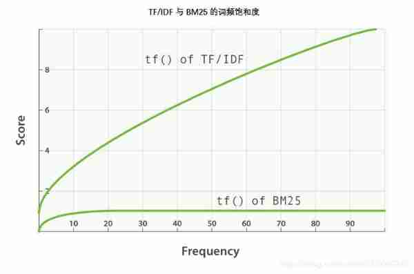
BM25 There is an upper limit , In the document 5 To 10 Words that appear only once or twice have a significant impact on the degree of correlation . But as shown here TF/IDF And BM25 Word frequency saturation See , Appears in the document 20 The words of times have almost the same influence as those that appear thousands of times .

2. Statistical indicators

2.1 Cosine Similarity

Cosine distance , Also known as cosine similarity , The cosine of the angle between two vectors in vector space is used as a measure of the difference between two individuals .Cosine Similarity The greater the absolute value of , The more similar the two vectors are , The value is negative. , Two vectors are negatively correlated .
$$CosineSimilarity(X,Y)=\frac{{\sum }_{i=1}^n{x}_i{y}_i}{\sqrt{{\sum }_{i=1}^n{x}_i^2}\sqrt{{\sum }_{i=1}^n{y}_i^2}}$$
Cosine similarity is more about distinguishing differences in direction , It's not sensitive to absolute values , Therefore, it is impossible to measure the difference of values in each dimension , Will lead to such a situation ：

Users rate content , Press 5 " ,X and Y Two users rated the two contents as （1,2） and （4,5）, The result of cosine similarity is 0.98, The two are very similar . But in terms of the score X Don't seem to like 2 This Content , and Y I prefer , The insensitivity of cosine similarity to numerical value results in the error of results , The irrationality needs to be corrected to adjust cosine similarity , That is, all the values in all dimensions are subtracted from a mean value , such as X and Y The average score is 3, Then adjust it to （-2,-1） and （1,2）, And then calculate the cosine similarity , obtain -0.8, The similarity is negative and the difference is not small , But it's obviously more realistic .

Adjust cosine similarity （Adjusted Cosine Similarity）：
$$AdjustedCosineSimilarity(X,Y)=\frac{{\sum }_{i=1}^n(x_i-\frac{1}{n}{\sum }_{i=1}^n{x}_i)(y_i-\frac{1}{n}{\sum }_{i=1}^n{y}_i)}{\sqrt{{\sum }_{i=1}^n(x_i-\frac{1}{n}{\sum }_{i=1}^n{x}_i{)}^2}\sqrt{{\sum }_{i=1}^n(y_i-\frac{1}{n}{\sum }_{i=1}^n{y}_i{)}^2}}$$

2.2 Jaccard Similarity

Jacquard coefficient , English is called Jaccard index, Also known as Jaccard similarity, It is used to compare the similarities and differences between finite sample sets .

Jaccard The larger the value of the coefficient , The higher the similarity of samples .

computing method ： The intersection of two samples divided by the union , When two samples are exactly the same , The result is 1, When two samples are completely different , The result is 0.

Range of calculation results ：$[0,1]$.
$$JaccardSimilarity(X,Y)=\frac{X\cap Y}{X\cup Y}$$
The opposite concept of the jacquard similarity coefficient is the jacquard distance （Jaccard Distance）, It can be expressed by the following formula ：
$$JaccardDistance(X,Y)=1-\frac{X\cap Y}{X\cup Y}$$
Jacquard distance measures the differentiation of two sets by the proportion of different elements in all elements .

2.3 Pearson Correlation

Pearson correlation coefficient (Pearson Correlation) It is defined as the quotient of covariance and standard deviation between two variables . It's actually a cosine similarity , But first we've centered the vector , Subtract the mean from each of the two vectors , Then calculate the cosine similarity . When the mean of both vectors is 0 when , Pearson's relative coefficient equals cosine similarity .

Range of calculation results ：$[-1,1]$,-1 It means negative correlation ,1 Ratio means positive correlation .

computing method ：
$$PearsonCorrelation(X,Y)=\frac{cov(X,Y)}{{\sigma }_X{\sigma }_Y}=\frac{{\sum }_{i=1}^n(X_i-\bar{X})(Y_i-\bar{Y})}{\sqrt{{\sum }_{i=1}^n(X_i-\bar{X}{)}^2}\sqrt{{\sum }_{i=1}^n(Y_i-\bar{Y}{)}^2}}$$

2.4 Euclidean Distance

Ming's distance （Minkowski Distance） Promotion of ：$p=1$ For Manhattan distance ,$p=2$ For Euclidean distance , Chebyshev distance is the form of the limit of Mings distance .
$$\begin{gathered} MinkowskiDistance=(\sum _{i=1}^n|x_i-y_i{|}^p{)}^{1/p} \\ ManhattanDistance=\sum _{i=1}^n|x_i-y_i| \\ EuclideanDistance=\sqrt{\sum _{i=1}^n(x_i-y_i{)}^2} \\ ChebyshevDistance=\underset{p\to \infty }{\lim }(\sum _{i=1}^n|x_i-y_i{|}^p{)}^{1/p}=\max |x_i-y_i| \end{gathered}$$
If the eigenvalues of two points are not in the same order of magnitude , Large eigenvalues will overwrite small ones . Such as Y1(10000,1),Y2(20000,2).

Standard Euclidean distance The idea of ： Standardize the data of each dimension ： Standardized value = ( Value before standardization － Mean value of components ) / Standard deviation of component , Then calculate the Euclidean distance .
$$StandardEuclideanDistance=\sqrt{\sum _{i=1}^n(\frac{x_i-y_i}{s_i}{)}^2}$$

3. Depth match

Reference resources

Common distance algorithm and similarity （ The correlation coefficient ） computing method

Deep learning to solve NLP problem ： Semantic similarity calculation

Similarity calculation method

Pluggable similarity algorithm

Welcome to my official account. 【SOTA Technology interconnection 】, I will share more dry goods .