当前位置:网站首页>Scanpy(七)基于scanorama整合scRNA-seq实现空间数据分析
Scanpy(七)基于scanorama整合scRNA-seq实现空间数据分析
2022-06-25 06:55:00 【tzc_fly】
本篇内容介绍如何使用多个Visium数据集,以及如何用scRNA-seq数据集进行整合。我们将使用Scanorama来进行整合。首先我们要安装Scanorama:
pip install scanorama
加载相关框架:
import scanpy as sc
import anndata as an
import pandas as pd
import numpy as np
import matplotlib as mpl
import matplotlib.pyplot as plt
import seaborn as sns
import scanorama

sc.logging.print_versions()
sc.set_figure_params(facecolor="white", figsize=(8, 8))
sc.settings.verbosity = 3

""" anndata 0.8.0 scanpy 1.9.1 scanorama 1.7.2 """
建议先阅读论文阅读笔记-利用Scanorama高效整合异质单细胞转录组
Reading the data
我们将使用两个小鼠大脑的Visium空间转录组数据集,该数据集可从10x genomics website获取。
函数datasets.visium_sge()从10x genomics下载数据集并返回adata对象(包含counts,images和spatial coordinates),我们使用pp.calculate_qc_metrics计算质量控制的指标,并做可视化。
adata_spatial_anterior = sc.datasets.visium_sge(
    sample_id="V1_Mouse_Brain_Sagittal_Anterior"
) # 数据集1
adata_spatial_posterior = sc.datasets.visium_sge(
    sample_id="V1_Mouse_Brain_Sagittal_Posterior"
) # 数据集2

adata_spatial_anterior
""" AnnData object with n_obs × n_vars = 2695 × 32285 obs: 'in_tissue', 'array_row', 'array_col' var: 'gene_ids', 'feature_types', 'genome' uns: 'spatial' obsm: 'spatial' """

adata_spatial_posterior
""" AnnData object with n_obs × n_vars = 3355 × 32285 obs: 'in_tissue', 'array_row', 'array_col' var: 'gene_ids', 'feature_types', 'genome' uns: 'spatial' obsm: 'spatial' """

adata_spatial_anterior.var_names_make_unique()
adata_spatial_posterior.var_names_make_unique()
sc.pp.calculate_qc_metrics(adata_spatial_anterior, inplace=True)
sc.pp.calculate_qc_metrics(adata_spatial_posterior, inplace=True)

for name, adata in [
    ("anterior", adata_spatial_anterior),
    ("posterior", adata_spatial_posterior),
]:
    fig, axs = plt.subplots(1, 4, figsize=(12, 3))
    fig.suptitle(f"Covariates for filtering: {
      name}")

    sns.distplot(adata.obs["total_counts"], kde=False, ax=axs[0])
    sns.distplot(
        adata.obs["total_counts"][adata.obs["total_counts"] < 20000],
        kde=False,
        bins=40,
        ax=axs[1],
    )
    sns.distplot(adata.obs["n_genes_by_counts"], kde=False, bins=60, ax=axs[2])
    sns.distplot(
        adata.obs["n_genes_by_counts"][adata.obs["n_genes_by_counts"] < 4000],
        kde=False,
        bins=60,
        ax=axs[3],
    )

sc.datasets.visium_sge下载的是已经过滤过的visium数据集,通过查看QC指标,我们可以观察到样本中几乎不包含空白点。
我们进一步对visium的counts数据进行标准化(使用内置的normalize_total函数),然后检测高变基因。
for adata in [
    adata_spatial_anterior,
    adata_spatial_posterior,
]:
    sc.pp.normalize_total(adata, inplace=True)
    sc.pp.log1p(adata)
    sc.pp.highly_variable_genes(adata, flavor="seurat", n_top_genes=2000, inplace=True)

""" normalizing counts per cell finished (0:00:00) If you pass `n_top_genes`, all cutoffs are ignored. extracting highly variable genes finished (0:00:00) --> added 'highly_variable', boolean vector (adata.var) 'means', float vector (adata.var) 'dispersions', float vector (adata.var) 'dispersions_norm', float vector (adata.var) normalizing counts per cell finished (0:00:00) If you pass `n_top_genes`, all cutoffs are ignored. extracting highly variable genes finished (0:00:00) --> added 'highly_variable', boolean vector (adata.var) 'means', float vector (adata.var) 'dispersions', float vector (adata.var) 'dispersions_norm', float vector (adata.var) """
查看两个数据集:
adata_spatial_anterior

""" AnnData object with n_obs × n_vars = 2695 × 32285 obs: 'in_tissue', 'array_row', 'array_col', 'n_genes_by_counts', 'log1p_n_genes_by_counts', 'total_counts', 'log1p_total_counts', 'pct_counts_in_top_50_genes', 'pct_counts_in_top_100_genes', 'pct_counts_in_top_200_genes', 'pct_counts_in_top_500_genes' var: 'gene_ids', 'feature_types', 'genome', 'n_cells_by_counts', 'mean_counts', 'log1p_mean_counts', 'pct_dropout_by_counts', 'total_counts', 'log1p_total_counts', 'highly_variable', 'means', 'dispersions', 'dispersions_norm' uns: 'spatial', 'log1p', 'hvg' obsm: 'spatial' """

adata_spatial_posterior

""" AnnData object with n_obs × n_vars = 3355 × 32285 obs: 'in_tissue', 'array_row', 'array_col', 'n_genes_by_counts', 'log1p_n_genes_by_counts', 'total_counts', 'log1p_total_counts', 'pct_counts_in_top_50_genes', 'pct_counts_in_top_100_genes', 'pct_counts_in_top_200_genes', 'pct_counts_in_top_500_genes' var: 'gene_ids', 'feature_types', 'genome', 'n_cells_by_counts', 'mean_counts', 'log1p_mean_counts', 'pct_dropout_by_counts', 'total_counts', 'log1p_total_counts', 'highly_variable', 'means', 'dispersions', 'dispersions_norm' uns: 'spatial', 'log1p', 'hvg' obsm: 'spatial' """
Data integration
现在,我们已经准备好对这两个数据集进行整合。如前所述,我们将使用Scanorama实现这一点。Scanorama返回包含两个adata的列表(每个adata包含了整合后的embedding)。关于数据整合,我们也可以使用BBKNN或Ingest。
adatas = [adata_spatial_anterior, adata_spatial_posterior]
adatas_cor = scanorama.correct_scanpy(adatas, return_dimred=True)

adatas_cor
""" [AnnData object with n_obs × n_vars = 2695 × 32285 obs: 'in_tissue', 'array_row', 'array_col', 'n_genes_by_counts', 'log1p_n_genes_by_counts', 'total_counts', 'log1p_total_counts', 'pct_counts_in_top_50_genes', 'pct_counts_in_top_100_genes', 'pct_counts_in_top_200_genes', 'pct_counts_in_top_500_genes' var: 'gene_ids', 'feature_types', 'genome', 'n_cells_by_counts', 'mean_counts', 'log1p_mean_counts', 'pct_dropout_by_counts', 'total_counts', 'log1p_total_counts', 'highly_variable', 'means', 'dispersions', 'dispersions_norm' uns: 'spatial', 'log1p', 'hvg' obsm: 'spatial', 'X_scanorama', AnnData object with n_obs × n_vars = 3355 × 32285 obs: 'in_tissue', 'array_row', 'array_col', 'n_genes_by_counts', 'log1p_n_genes_by_counts', 'total_counts', 'log1p_total_counts', 'pct_counts_in_top_50_genes', 'pct_counts_in_top_100_genes', 'pct_counts_in_top_200_genes', 'pct_counts_in_top_500_genes' var: 'gene_ids', 'feature_types', 'genome', 'n_cells_by_counts', 'mean_counts', 'log1p_mean_counts', 'pct_dropout_by_counts', 'total_counts', 'log1p_total_counts', 'highly_variable', 'means', 'dispersions', 'dispersions_norm' uns: 'spatial', 'log1p', 'hvg' obsm: 'spatial', 'X_scanorama'] """

len(adatas_cor) # 2
adatas_cor[0].obsm['X_scanorama'].shape # (2695, 100)
然后,我们拼接整合后的embedding,整合后的数据集为adata_spatial,embedding保存为adata_spatial.obsm['scanorama_embedding']。此外,我们将计算UMAP以可视化结果并定性评估数据整合任务。
请注意,我们使用uns_merge="unique"策略连接两个数据集,这是为了在连接的anndata对象中保留visium数据集中的两个images。
adata_spatial = sc.concat(
    adatas_cor,
    label="library_id",
    uns_merge="unique",
    keys=[
        k
        for d in [
            adatas_cor[0].uns["spatial"],
            adatas_cor[1].uns["spatial"],
        ]
        for k, v in d.items()
    ],
    index_unique="-",
)

sc.pp.neighbors(adata_spatial, use_rep="X_scanorama")
sc.tl.umap(adata_spatial)
sc.tl.leiden(adata_spatial, key_added="clusters")
""" computing neighbors finished: added to `.uns['neighbors']` `.obsp['distances']`, distances for each pair of neighbors `.obsp['connectivities']`, weighted adjacency matrix (0:00:06) computing UMAP finished: added 'X_umap', UMAP coordinates (adata.obsm) (0:00:09) running Leiden clustering finished: found 22 clusters and added 'clusters', the cluster labels (adata.obs, categorical) (0:00:00) """

adata_spatial
""" AnnData object with n_obs × n_vars = 6050 × 32285 obs: 'in_tissue', 'array_row', 'array_col', 'n_genes_by_counts', 'log1p_n_genes_by_counts', 'total_counts', 'log1p_total_counts', 'pct_counts_in_top_50_genes', 'pct_counts_in_top_100_genes', 'pct_counts_in_top_200_genes', 'pct_counts_in_top_500_genes', 'library_id', 'clusters' uns: 'spatial', 'log1p', 'hvg', 'neighbors', 'umap', 'leiden' obsm: 'spatial', 'X_scanorama', 'X_umap' obsp: 'distances', 'connectivities' """

sc.pl.umap(
    adata_spatial, color=["clusters", "library_id"], palette=sc.pl.palettes.default_20
)

我们还可以在空间坐标中可视化聚类结果。为此,我们首先需要将簇颜色保存在字典中。然后,我们可以在前后两个数据集的视图中可视化,并将结果并排显示。
clusters_colors = dict(
    zip([str(i) for i in range(18)], adata_spatial.uns["clusters_colors"])
)

fig, axs = plt.subplots(1, 2, figsize=(15, 10))

for i, library in enumerate(
    ["V1_Mouse_Brain_Sagittal_Anterior", "V1_Mouse_Brain_Sagittal_Posterior"]
):
    ad = adata_spatial[adata_spatial.obs.library_id == library, :].copy()
    sc.pl.spatial(
        ad,
        img_key="hires",
        library_id=library,
        color="clusters",
        size=1.5,
        palette=[
            v
            for k, v in clusters_colors.items()
            if k in ad.obs.clusters.unique().tolist()
        ],
        legend_loc=None,
        show=False,
        ax=axs[i],
    )

plt.tight_layout()

从这些簇中,我们可以清楚地看到两种组织中的分层。这证明,数据集整合确实工作正确。
边栏推荐
- Use pytorch to build mobilenetv2 and learn and train based on migration
- VOCALOID notes
- CVPR 2022 oral 2D images become realistic 3D objects in seconds
- [supplementary question] 2021 Niuke summer multi school training camp 9-N
- STM32CubeMX 學習(5)輸入捕獲實驗
- Wechat applet opening customer service message function development
- 現在通過開戶經理發的開戶鏈接股票開戶安全嗎?
- [supplementary question] 2021 Niuke summer multi school training camp 6-n
- The difference between personal domain name and enterprise domain name
- Common action types
猜你喜欢
共话云原生数据库的未来

C examples of using colordialog to change text color and fontdialog to change text font

初体验完全托管型图数据库 Amazon Neptune

In 2022, which industry will graduates prefer when looking for jobs?

Electronics: Lesson 010 - Experiment 9: time and capacitors
![[QT] QT 5 procedure: print documents](/img/76/2fce505c43f75360a8ff477aa2d31d.png)
[QT] QT 5 procedure: print documents
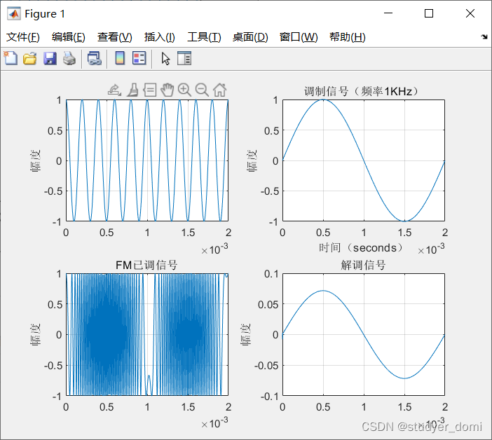
FM signal, modulated signal and carrier

Authority design of SaaS system based on RBAC

测一测现在的温度

Opencv daily function structure analysis and shape descriptor (8) Fitline function fitting line
随机推荐
Electronics: Lesson 013 - Experiment 14: Wearable pulsed luminaries
电子学:第013课——实验 14:可穿戴的脉冲发光体
Rqt command
电子学:第010课——实验 8:继电振荡器
FFT [template]
Authority design of SaaS system based on RBAC
[supplementary question] 2021 Niuke summer multi school training camp 1-3
Stm32cubemx Learning (5) Input capture Experiment
牛客:飞行路线(分层图+最短路)
STM32CubeMX 學習(5)輸入捕獲實驗
Go语言学习教程(十三)
Not afraid of losing a hundred battles, but afraid of losing heart
June training (day 25) - tree array
DNS protocol and its complete DNS query process
How to create a new branch with SVN
Log in to MySQL 5.7 under ubuntu18 and set the root password
PHP array function Encyclopedia
Basic record of getting started with PHP
Use pytorch to build mobilenetv2 and learn and train based on migration
现在通过开户经理发的开户链接股票开户安全吗?