8. Intelligent transportation project (1)

brief introduction

Environmental Science

NumPy  It's using  Python  The basic package for Scientific Computing .

Numba  It's open source  JIT  compiler , It will  Python  and  NumPy  A subset of the code is converted to fast machine code .

SciPy  Is mathematics 、 Open source software for science and Engineering .SciPy  The library depends on  NumPy, It provides convenient and fast  N  Dimension array operations .

h5py  from  Python  Read and write  HDF5 file .

pandas  For data analysis 、 Powerful data structure for time series and statistics .

opencv-python  be used for  Python  Pre construction of  OpenCV  package .

moviepy  Toolkit for video processing 

Filterpy  Kalman filter and particle filter are realized 

 conda create -n CGLearnIng36 python=3.6

amqp==2.5.2
billiard==3.6.3.0
celery==4.4.2
certifi==2019.11.28
chardet==3.0.4
click==7.1.1
colorama==0.3.9
cycler==0.10.0
Cython==0.29.4
decorator==4.4.2
Django==2.2.10
django-redis==4.11.0
filterpy==1.4.5
fire==0.1.3
Flask==1.1.1
h5py==2.8.0
idna==2.8
imageio==2.8.0
imageio-ffmpeg==0.4.1
importlib-metadata==1.6.0
imutils==0.5.3
itsdangerous==1.1.0
Jinja2==2.11.1
Kalman==0.1.3
kiwisolver==1.1.0
kombu==4.6.8
llvmlite==0.31.0
MarkupSafe==1.1.1
matplotlib==2.2.3
moviepy==1.0.1
numba==0.39.0
numpy==1.15.4
opencv-python==3.4.3.18
pandas==0.23.4
Pillow==7.0.0
proglog==0.1.9
protobuf==3.11.3
pyparsing==2.4.6
python-dateutil==2.8.1
pytz==2019.3
redis==3.4.1
requests==2.21.0
scipy==1.1.0
six==1.14.0
sqlparse==0.3.1
tensorboardX==1.6
torch==0.4.1
torchvision==0.2.1
tqdm==4.29.1
urllib3==1.24.3
vine==1.3.0
Werkzeug==1.0.0
zipp==3.1.0

numba

numba Is a program for compiling Python Compilers for arrays and numeric functions , This compiler can greatly improve direct use Python The operation speed of the function written .
numba Use LLVM The compiler architecture will be pure Python Code generation optimized machine code , Add simple comments through a few , Will be array oriented and use a lot of math python Code optimized to match c,c++ and Fortran Similar performance , Without changing Python Interpreter .numba The compilation method of is shown in the following figure ：

Although there are cython and Pypy And many other compilers , choice Numbade The reason is simple , You don't have to leave python Code comfort zone , You don't need to change your code to get some acceleration , We just need to add a decorator to Python Function to complete the acceleration , And the acceleration effect is similar to cython The code is quite .

numba When accelerating code , Add... To the function to be optimized @jit The optimizer can . Use jit You can make numba To decide when and how to optimize . The following simple example shows ：

from numba import jit
@jit
def f(x, y):
    return x + y

The calculation of this code is performed for the first time when it is called ,numba Parameter types will be inferred during the call , Based on this information, the optimized code is generated .numba You can also compile and generate specific code based on the type of input . for example , For the above code , Passing in integers and floating-point numbers as parameters will generate different codes ：

Numba Compiled functions can call other compiled functions

@jit
def hypot(x, y):
    return math.sqrt(square(x) + square(y))

from numba import jit
import time
@jit
def foo():
    x = []
    for a in range(100000000):
        x.append(a)

def foo_withoutfit():
    y = []  
    for b in range(100000000):
        y.append(b)

Now we define the same method , The functions implemented are the same , One is to make use of numba Accelerate , One without acceleration , Let's take a look at their running time ：

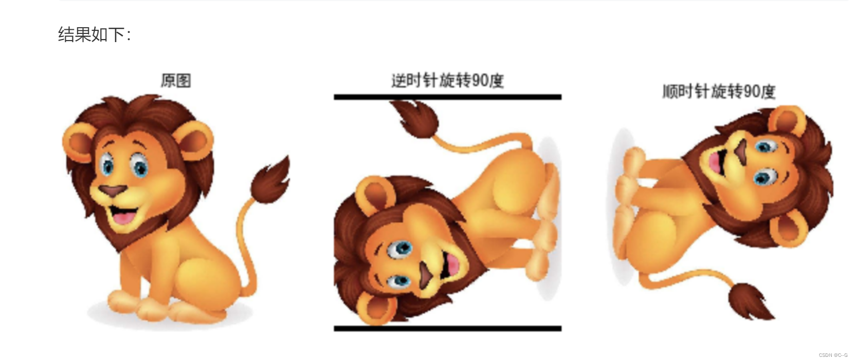
imutils

imutils Is in OPenCV Based on a package , To achieve a simpler call OPenCV Purpose of the interface , It can easily realize the translation of the image , rotate , The zoom , Skeleton and a series of operations .

• Image translation
  OpenCV The implementation of image translation is also provided in , First calculate the translation matrix , Then the affine transformation is used to realize translation , stay imutils You can translate the image directly in .

translated = imutils.translate(img,x,y)

• Image zoom
  Zoom the picture in OPenCV Care should be taken to ensure that the aspect ratio is maintained . And in the imutils The aspect ratio of the original image is automatically maintained in , Specify only the width weight and Height that will do .

img = cv.imread("lion.jpeg")
resized = imutils.resize(img,width=200)
print(" Original image size : ", img.shape)
print(" Scaled size ：",resized.shape)
plt.figure(figsize=[10, 10])
plt.subplot(1,2,1)
plt.imshow(cv.cvtColor(img, cv.COLOR_BGR2RGB))
plt.title(' Original picture ')
plt.axis("off")
plt.subplot(1,2,2)
plt.imshow(cv.cvtColor(resized, cv.COLOR_BGR2RGB))
plt.title(' Zoom results ')
plt.axis("off")
plt.show()

• Image rotation
  stay OpenCV Affine transformation is used for rotation in , The image rotation method here is imutils.rotate(), Follow 2 Parameters , The first is picture data , The second is the angle of rotation , Rotation is counterclockwise . meanwhile imutils Another similar approach is provided , rotate_round(), It just rotates clockwise .

import cv2
import imutils

image = cv2.imread('lion.jpeg')
rotated = imutils.rotate(image, 90)                                                                                      
rotated_round = imutils.rotate_bound(image, 90)                                 

plt.figure(figsize=[10, 10])
plt.subplot(1,3,1)
plt.imshow(img[:,:,::-1])
plt.title(' Original picture ')
plt.axis("off")
plt.subplot(1,3,2)
plt.imshow(rotated[:,:,::-1])
plt.title(' Counter clockwise rotation 90 degree ')
plt.axis("off")
plt.subplot(1,3,3)
plt.imshow(rotated_round[:,:,::-1])
plt.title(' Clockwise rotation 90 degree ')
plt.axis("off")
plt.show()

• Skeleton extraction
  Skeleton extraction , It refers to the topological skeleton of the objects in the picture (topological skeleton) The process of building .imutils The method provided is skeletonize(), The second parameter is the size of the structural parameter (structuring element), It is equivalent to a particle size , The smaller the size, the longer the processing time .

import cv2
import imutils
# 1  Image reading 
image = cv2.imread('lion.jpeg')
# 2  Graying 
gray = cv2.cvtColor(image, cv2.COLOR_BGR2GRAY)                                  
# 3  Skeleton extraction 
skeleton = imutils.skeletonize(gray, size=(3, 3))  
# 4  Image display 
plt.figure(figsize=(10,8),dpi=100)
plt.subplot(121),plt.imshow(img[:,:,::-1]),plt.title(' Original picture ')
plt.xticks([]), plt.yticks([])
plt.subplot(122),plt.imshow(skeleton,cmap="gray"),plt.title(' Skeleton extraction results ')
plt.xticks([]), plt.yticks([])
plt.show()

• Matplotlib Show
  stay OpenCV Of Python Binding , Image with BGR The order is expressed as NumPy Array . Use this cv2.imshow The function works very well . however , If you plan to use Matplotlib, The plt.imshow The function will assume that the image is pressed RGB Sequential arrangement . call cv2.cvtColor Solve this problem , You can also use opencv2matplotlib Convenient features .

img = cv.imread("lion.jpeg")
plt.figure()
plt.imshow(imutils.opencv2matplotlib(img))

• OPenCV Version detection
  OpenCV 4 After the release , With the update of the major version , Backward compatibility is particularly prominent . In the use of OPenCV when , You should check which version of... Is currently in use OpenCV, Then use the appropriate function or method . stay imutils Medium is_cv2()、is_cv3() and is_cv4() Can be used to automatically determine the current environment OpenCV Version of the simple features .

print("OPenCV edition : {}".format(cv2.__version__))
print("OPenCV yes 2.X? {}".format(imutils.is_cv2()))
print("OPenCV yes 3.X? {}".format(imutils.is_cv3()))
print("OPenCV yes 4.X? {}".format(imutils.is_cv4()))

cv.dnn

OPenCV since 3.3 Version start , Added support for deep learning networks , namely DNN modular , It supports mainstream deep learning framework generation and model loading everywhere .

• brief introduction

OpenCV Deep learning module in （DNN） It only provides reasoning function , Model training is not involved , Support multiple deep learning frameworks , such as TensorFlow,Caffe,Torch and Darknet.

• framework
  
  In addition to the above acceleration methods ,DNN The module also has network level optimization . There are two types of optimization , One is layer fusion , There is also memory reuse .
  
  
  

• Common methods

dnn.blobFromImage
effect ： According to the input image , Create dimensions N（ The number of pictures ）, The channel number C, high H And width W Sequential blobs

blobFromImage(image, 
                  scalefactor=None, 
                  size=None, 
                  mean=None, 
                  swapRB=None, 
                  crop=None, 
                  ddepth=None):

import cv2
from cv2 import dnn
import numpy as np 
import matplotlib.pyplot as plt

img_cv2 = cv2.imread("test.jpeg")
print(" Original image size : ", img_cv2.shape)

inWidth = 256
inHeight = 256
outBlob1 = cv2.dnn.blobFromImage(img_cv2,
                                scalefactor=1.0 / 255,
                                size=(inWidth, inHeight),
                                mean=(0, 0, 0),
                                swapRB=False,
                                crop=False)
print(" Uncut output : ", outBlob1.shape)
outimg1 = np.transpose(outBlob1[0], (1, 2, 0))

outBlob2 = cv2.dnn.blobFromImage(img_cv2,
                                scalefactor=1.0 / 255,
                                size=(inWidth, inHeight),
                                mean=(0, 0, 0),
                                swapRB=False,
                                crop=True)
print(" Crop output : ", outBlob2.shape)
outimg2 = np.transpose(outBlob2[0], (1, 2, 0))

plt.figure(figsize=[10, 10])
plt.subplot(1, 3, 1)
plt.title(' The input image ', fontsize=16)
plt.imshow(cv2.cvtColor(img_cv2, cv2.COLOR_BGR2RGB))
plt.axis("off")
plt.subplot(1, 3, 2)
plt.title(' Output image  -  Not cut ', fontsize=16)
plt.imshow(cv2.cvtColor(outimg1, cv2.COLOR_BGR2RGB))
plt.axis("off")
plt.subplot(1, 3, 3)
plt.title(' Output image  -  tailoring ', fontsize=16)
plt.imshow(cv2.cvtColor(outimg2, cv2.COLOR_BGR2RGB))
plt.axis("off")
plt.show()

Another one API With the above API similar , It is used for batch image processing

blobFromImages(images, 
                   scalefactor=None, 
                   size=None, mean=None, 
                   swapRB=None, 
                   crop=None, 
                   ddepth=None):

effect ： Batch processing pictures , establish 4 Dimensional blob, Other parameters are similar to dnn.blobFromImage

.dnn.NMSBoxes
effect ： According to the given detection boxes And corresponding scores Conduct NMS（ Non maximum suppression ） Handle

NMSBoxes(bboxes, 
             scores, 
             score_threshold, 
             nms_threshold, 
             eta=None, 
             top_k=None)

dnn.readNet
effect ： Load the deep learning network and its model parameters

readNet(model, config=None, framework=None)

Corresponding to a specific framework API：

Caffe

readNetFromCaffe(prototxt, caffeModel=None)

effect ： Load with Caffe Configuration network and training weight parameters
Darknet

readNetFromDarknet(cfgFile, darknetModel=None)

effect ： Load with Darknet Configuration network and training weight parameters

Tensorflow

readNetFromTensorflow(model, config=None)

effect ： Load with Tensorflow Configuration network and training weight parameters

Parameters ：

 - model: .pb  file 

 - config: .pbtxt  file 

Torch

readNetFromTorch(model, isBinary=None)

effect ： Load with Torch Configuration network and training weight parameters

Parameters ：

 - model:  use  torch.save() File saved by function 

ONNX

readNetFromONNX(onnxFile)

effect ： load .onnx Model network configuration parameters and weight parameters

Traffic flow detection

Multi target tracking

Multi target tracking classification

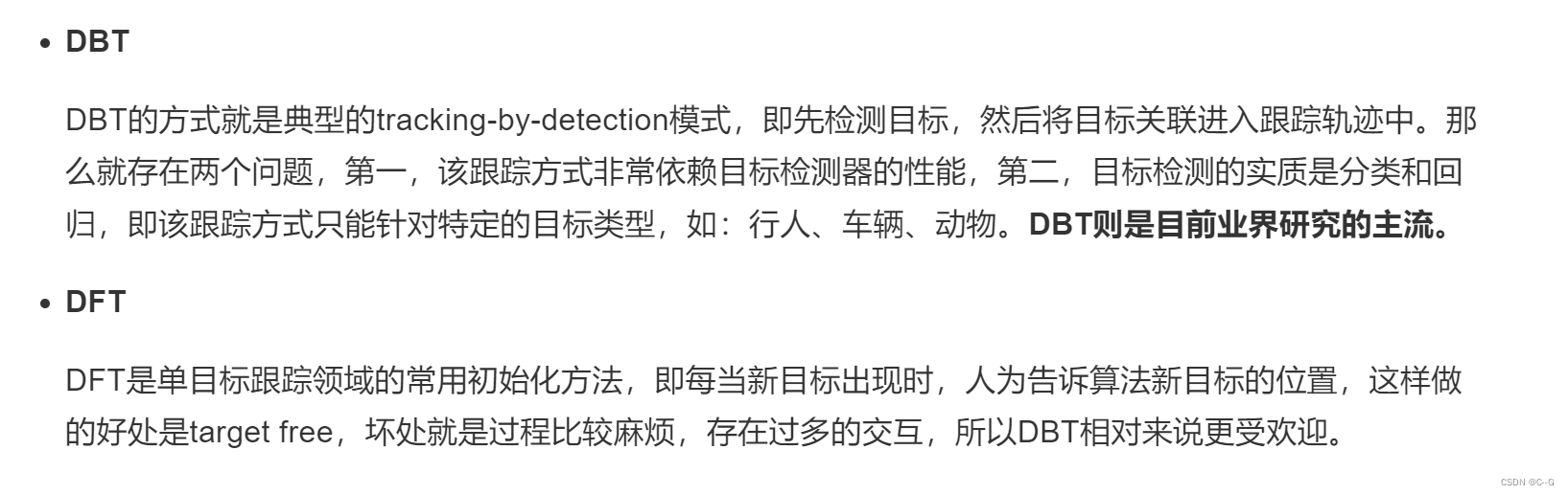
Multitarget tracking , namely MOT（Multi-Object Tracking）, That is to track multiple targets in a video at the same time .MOT It is mainly used in the fields of security monitoring and automatic driving .

• Initialization method
  In the multi-target tracking problem, not all targets will appear in the first frame , Not all targets will appear in every frame . How to initialize the target that appears , It can be used as the classification pointer of tracking algorithm . Common initialization methods fall into two categories , One is Detection-Based-Tracking(DBT), One is Detection-Free-Tracking(DFT). The following figure vividly illustrates the difference between the two types of algorithms .
  
  
• Processing mode
  MOT There are also different processing modes ,Online and Offline Two categories: , The main difference is whether the information of subsequent frames is used . The figure below illustrates Online And Offline The difference between tracking .
  
  

Motion models

In order to simplify the difficulty of multi-target tracking , We introduce the motion model class to simplify the solution process , The motion model captures the dynamic behavior of the target , It estimates the potential position of the target in the future frame , So as to reduce the search space . in the majority of cases , Suppose the target is moving smoothly in reality , So the same is true in image space . For the movement of the vehicle , It can be roughly divided into linear motion and nonlinear motion ：

• Linear motion ： Linear motion model is the most popular model at present , That is, the motion attribute of the target is assumed to be stable （ Speed , The acceleration , Location ）;
• Nonlinear motion ： Although linear motion models are commonly used , But because of the problems that it cannot solve , The nonlinear motion model was born . It can make tracklets The calculation of motion similarity is more accurate .

Tracking method

Algorithm based on neural network in multi-target tracking , There are not many end-to-end algorithms , It's still in the list brushing stage in the laboratory , Complex model , Slow speed , The tracking results are not good , We won't introduce it anymore , We mainly introduce the following two mainstream algorithms ：

• be based on Kalman and KM Back end optimization algorithm of the algorithm
  This kind of algorithm can achieve real-time performance , But depending on the detection algorithm, the effect is better , Feature differentiation is better （ The output of the final result depends on a strong detection algorithm , The tracking algorithm based on Kalman and Hungarian matching can output the information of the detected target id, Secondly, it can ensure the real-time performance of the tracking algorithm ）, The tracking effect will be good ,id Less switching . The representative algorithm is SORT/DeepSORT.
  
  SORT It is a practical multi-target tracking algorithm , Linear velocity model and Kalman filter are introduced to predict the position , In the absence of an appropriate match detection frame , Use motion models to predict the position of objects . Hungary algorithm is an algorithm for finding the maximum matching of bipartite graph , In the multi-target tracking problem, it can be simply understood as an algorithm to find the matching optimal solution of several targets in the two frames . And Kalman filter can be regarded as a kind of motion model , Used to predict the trajectory of a target , And use the tracking results with high confidence to correct the prediction results .

Multi - target tracking is usually followed by target detection . In the industrial world, target detection is more commonly used yolo Detection network , Single stage , Fast , The accuracy is not bad , Deployed in NV The platform frame rate can reach 30fps above . Therefore, it is necessary to realize the task of integrating target detection code and multi-target tracking code , We need to unify the framework of both . First, realize the target detection network , The output result of the detection is mainly to input the position information of the detection box into the multi-target tracking algorithm .

• Multitarget tracking algorithm based on multithread single target tracking
  This kind of algorithm is characterized by good tracking effect , Because it assigns a tracker to each class of objects . However, the algorithm requires a large change of target scale , Parameter debugging needs to be reasonable , At the same time, the algorithm consumes cpu resources , Real time is not high , The representative algorithm is to use KCF Target tracking .

In essence, multi-target tracking is the problem of multiple targets moving at the same time , Therefore, the problem of introducing single target tracker into multi-target tracking has been put forward , Assign a tracker to each target , Then, the matching algorithm is used indirectly to correct those failed tracking or new targets . The typical single target tracking algorithm is kernel correlation filtering algorithm （KCF）, It can reach a very high level both in accuracy and speed , It was one of the best algorithms for single target tracking at that time , Many single target tracking algorithms have been improved based on this .

In the actual application process, each target will be assigned a KCF Trackers and organize these trackers in a multi-threaded way . At the same time, due to the limitation of actual hardware conditions , It is impossible to provide powerful computing power resources , The tracking strategy of alternating detector and tracker will be adopted . Because the detected frame rate is not high , It makes the maintenance effect of tracking lag or frame drift more serious , Not very practical .

Auxiliary function

IOU It's Cross and compare （Intersection-over-Union） A concept used in object detection is the generation of candidate boxes （candidate bound） Same as the original marker box （ground truth bound） Overlap rate of , That is, the ratio of their intersection to Union . Ideally, complete overlap , That is, the ratio is 1. In multi-target tracking , It is used to distinguish the similarity between the tracking frame and the target detection frame .

Calculate the ratio of intersection and union

oU Is the intersection of two regions divided by two regions and the result is

def iou(bb_test, bb_gt):
    """  In two box Inter calculation IOU :param bb_test: box1 = [x1y1x2y2] :param bb_gt: box2 = [x1y1x2y2] :return:  Occurring simultaneously than IOU """
    xx1 = np.maximum(bb_test[0], bb_gt[0])
    yy1 = np.maximum(bb_test[1], bb_gt[1])
    xx2 = np.minimum(bb_test[2], bb_gt[2])
    yy2 = np.minimum(bb_test[3], bb_gt[3])
    w = np.maximum(0., xx2 - xx1)
    h = np.maximum(0., yy2 - yy1)
    wh = w * h
    o = wh / ((bb_test[2] - bb_test[0]) * (bb_test[3] - bb_test[1]) + (bb_gt[2] - bb_gt[0]) * (
            bb_gt[3] - bb_gt[1]) - wh)
    return o

The representation of the candidate box

• Convert the candidate box from coordinate form to center point coordinate and area form

def convert_bbox_to_z(bbox):
    """  take [x1,y1,x2,y2] The detection frame of the form is transformed into the state representation of the filter [x,y,s,r]. among x,y Is the central coordinate of the frame ,s It's the area , scale ,r It's the aspect ratio  :param bbox: [x1,y1,x2,y2]  They are the upper left corner coordinates and the lower right corner coordinates  :return: [ x, y, s, r ] 4 That's ok 1 Column , among x,y yes box Coordinates of the center position ,s It's the area ,r Is the aspect ratio w/h """
    w = bbox[2] - bbox[0]
    h = bbox[3] - bbox[1]
    x = bbox[0] + w / 2.
    y = bbox[1] + h / 2.
    s = w * h
    r = w / float(h)
    return np.array([x, y, s, r]).reshape((4, 1))

• Convert the candidate box from the form of central area to the form of coordinates

def convert_x_to_bbox(x, score=None):
    """  take [cx,cy,s,r] The target box of indicates to turn to [x_min,y_min,x_max,y_max] In the form of  :param x:[ x, y, s, r ], among x,y yes box Coordinates of the center position ,s It's the area ,r :param score:  Degree of confidence  :return:[x1,y1,x2,y2], Top left and bottom right coordinates  """
    w = np.sqrt(x[2] * x[3])
    h = x[2] / w
    if score is None:
        return np.array([x[0] - w / 2., x[1] - h / 2., x[0] + w / 2., x[1] + h / 2.]).reshape((1, 4))
    else:
        return np.array([x[0] - w / 2., x[1] - h / 2., x[0] + w / 2., x[1] + h / 2., score]).reshape((1, 5))

Kalman filter

brief introduction

Kalman filtering （Kalman） It is a common algorithm in both single target and multi-target fields , We regard Kalman filter as a motion model , Used to predict the position of the target , And use the prediction results to correct the tracked target , It belongs to a method of automatic control theory .

When tracking the target in the video , When the target moves slowly , It is easy to associate the targets of the previous and subsequent frames , As shown in the figure below :

If the target moves faster , Or when performing inter frame detection , In subsequent frames , The goal is A Has moved to the previous frame B Where it is , At this time, the association will get the wrong result , take A‘ And B Link together .

So how can we avoid this kind of correlation error ？ We can do this before we do the target correlation , Predict the position of the target in subsequent frames , And then compare with the predicted results , As shown in the figure below ：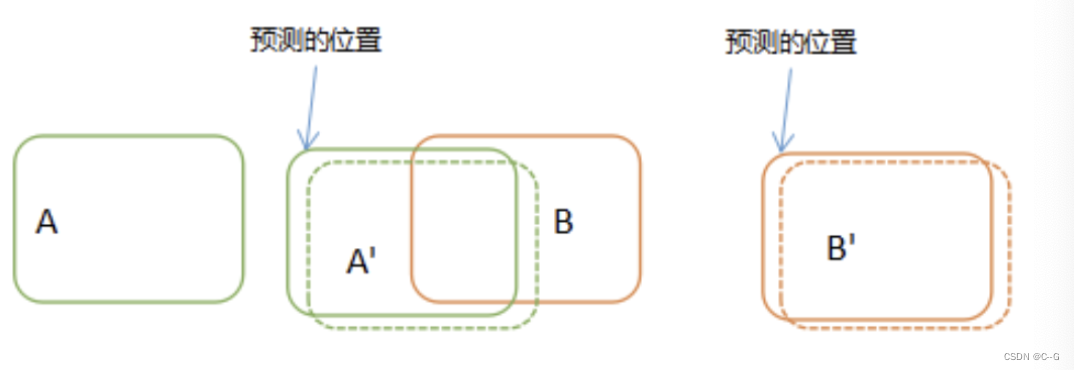

Before we compare the correlations , First predict A and B Position in the next frame , Then the actual detection position is compared with the predicted position , As long as the forecast is accurate enough , There is almost no error due to the speed .

Kalman filter can be used to predict the position of the target in subsequent frames , As shown in the figure below , The Kalman filter can determine the position of the target according to the data of the previous five frames , Forecast No 6 The position of the frame target .

The biggest advantage of Kalman filter is to use recursive method to solve the problem of linear filtering , It only needs the current measured value and the predicted value of the previous cycle to estimate the state . Because this recursive method does not need a lot of storage space , The calculation amount of each step is small , The calculation steps are clear , Very suitable for computer processing , So Kalman filter has been widely welcomed , It has broad application prospects in various fields .

principle

Let's assume a simple scenario , There is a small car running , Its speed is v, Its position can be observed p, In other words, we can observe the status of the car in real time .

• Scene description
  

Although we are quite sure of the car's state at this time , There will be some errors in both calculation and detection , So we can only think that the current state is an optimal estimate of its real state . Then we may consider that the current state obeys a Gaussian distribution , As shown in the figure below ：

• Predict the state of the next moment
  Now we need to go through the current status of the car , Use some knowledge of physics to predict its next state , That is, through k-1 The position and speed of the moment , It can be inferred that the state of the next moment is ：
  
  

• Increase the internal control of the system
  We need to control the car , Like acceleration and deceleration , Suppose the acceleration we apply at some point is \color{green}{\mathbf{a}}a, Then the position and speed at the next moment should be :
  
  

• Consider the external influence of the system
  

• Prediction of observed data
  We passed the previous state of the car , Its current state is predicted , At this point, we should consider what can be observed about the state of the car ？
  

• Actual observations
  It is speculated that the current status of the trolley , Extrapolated our observations , But there must be a gap between reality and ideal , Our predicted observation results and actual observation results may be as shown in the figure below ：
  
  
  The most important and core thing that Kalman filter needs to do is to fuse the results of prediction and observation , Make full use of the uncertainty of both to get more accurate estimates . Generally speaking, it is how to get the Gaussian distribution of the middle light yellow part from the two ellipses above , It seems that this is the coincidence of the predicted and observed Gaussian distributions , That is, the part with high probability .

• Product of Gaussian distribution
  For any two Gaussian distributions , After multiplying the two, it is still Gaussian distribution , We use two properties of Gaussian distribution to solve , One is that the distribution function at the mean value takes the maximum value , The second is that the curvature of the distribution curve at the mean value is the second derivative , We can work out ：
  
  
  The direct product of the blue and orange waveforms in the figure is the Yellow waveform , Purple is a demerit that calculates the mean and variance , The Yellow distribution can be obtained by multiplying the purple waveform by a coefficient .
  

• New Gaussian distribution
  The product of the Gaussian distribution of the prediction and the observed value is the optimal estimation of the Kalman filter ：
  
  

• The calculation method in practice
  

Kalman filter practice

filterpy

FilterPy Is a realization of a variety of filters Python modular , It implements the famous Kalman filter and particle filter . We can directly call the library to complete the implementation of Kalman filter . The main modules include ：

Open source code

• initialization
  Preset state variables dim_x And observation variable dimension dim_z、 Covariance matrix P、 Motion form and observation matrix H etc. , Generally, each covariance matrix will be initialized as an identity matrix , Corresponding settings are required according to specific scenarios .

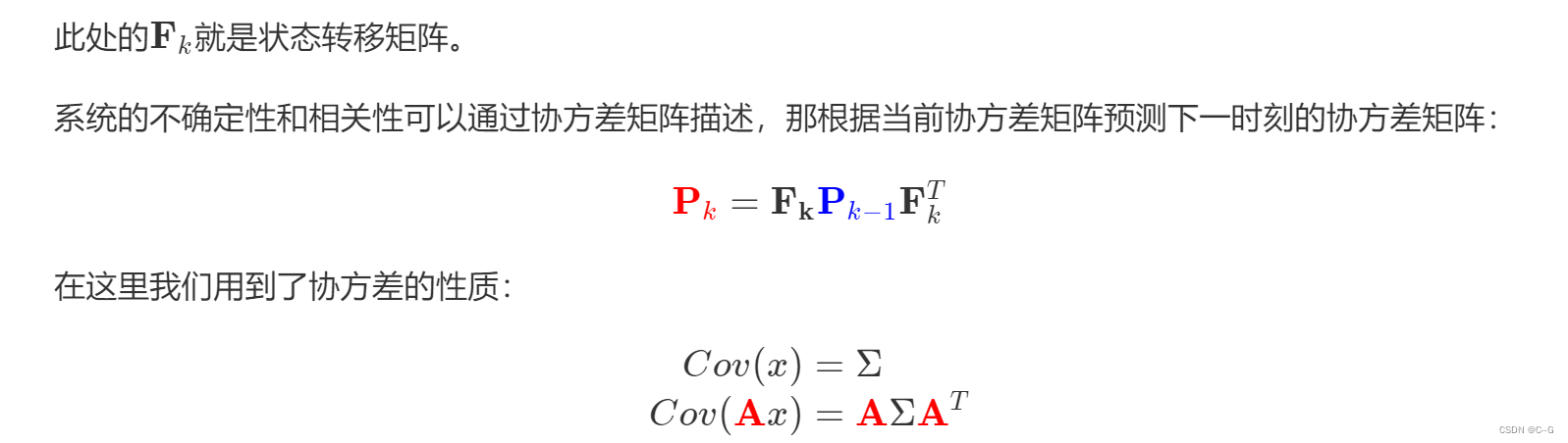
def __init__(self, dim_x, dim_z, dim_u = 0, x = None, P = None,
             Q = None, B = None, F = None, H = None, R = None):
    """Kalman Filter Refer to http:/github.com/rlabbe/filterpy Method ----------------------------------------- Predict | Update ----------------------------------------- | K = PH^T(HPH^T + R)^-1 x = Fx + Bu | y = z - Hx P = FPF^T + Q | x = x + Ky | P = (1 - KH)P | S = HPH^T + R ----------------------------------------- note: In update unit, here is a more numerically stable way: P = (I-KH)P(I-KH)' + KRK' Parameters ---------- dim_x: int dims of state variables, eg:(x,y,vx,vy)->4 dim_z: int dims of observation variables, eg:(x,y)->2 dim_u: int dims of control variables,eg: a->1 p = p + vt + 0.5at^2 v = v + at =>[p;v] = [1,t;0,1][p;v] + [0.5t^2;t]a """

    assert dim_x >= 1, 'dim_x must be 1 or greater'
    assert dim_z >= 1, 'dim_z must be 1 or greater'
    assert dim_u >= 0, 'dim_u must be 0 or greater'

    self.dim_x = dim_x
    self.dim_z = dim_z
    self.dim_u = dim_u

    # initialization
    # predict
    self.x = np.zeros((dim_x, 1)) if x is None else x      # state
    self.P = np.eye(dim_x)  if P is None else P            # uncertainty covariance
    self.Q = np.eye(dim_x)  if Q is None else Q            # process uncertainty for prediction
    self.B = None if B is None else B                      # control transition matrix
    self.F = np.eye(dim_x)  if F is None else F            # state transition matrix

    # update
    self.H = np.zeros((dim_z, dim_x)) if H is None else H  # Measurement function z=Hx
    self.R = np.eye(dim_z)  if R is None else R            # observation uncertainty
    self._alpha_sq = 1.                              # fading memory control
    self.z = np.array([[None] * self.dim_z]).T       # observation
    self.K = np.zeros((dim_x, dim_z))                # kalman gain
    self.y = np.zeros((dim_z, 1))                    # estimation error
    self.S = np.zeros((dim_z, dim_z))                # system uncertainty, S = HPH^T + R
    self.SI = np.zeros((dim_z, dim_z))               # inverse system uncertainty, SI = S^-1

    self.inv = np.linalg.inv
    self._mahalanobis = None                         # Mahalanobis distance of measurement
    self.latest_state = 'init'                       # last process name

• Prediction stage
  Next, let's move on to the prediction process , To ensure versatility , Forgetting coefficient is introduced α, Its role is to adjust the degree of dependence on past information ,α The greater the dependence on historical information, the less ：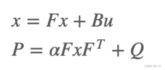
  

def predict(self, u = None, B = None, F = None, Q = None):
    """ Predict next state (prior) using the Kalman filter state propagation equations: x = Fx + Bu P = fading_memory*FPF^T + Q Parameters ---------- u : ndarray Optional control vector. If not `None`, it is multiplied by B to create the control input into the system. B : ndarray of (dim_x, dim_z), or None Optional control transition matrix; a value of None will cause the filter to use `self.B`. F : ndarray of (dim_x, dim_x), or None Optional state transition matrix; a value of None will cause the filter to use `self.F`. Q : ndarray of (dim_x, dim_x), scalar, or None Optional process noise matrix; a value of None will cause the filter to use `self.Q`. """

    if B is None:
        B = self.B
    if F is None:
        F = self.F
    if Q is None:
        Q = self.Q
    elif np.isscalar(Q):
        Q = np.eye(self.dim_x) * Q

    # x = Fx + Bu
    if B is not None and u is not None:
        self.x = F @ self.x + B @ u
    else:
        self.x = F @ self.x

    # P = fading_memory*FPF' + Q
    self.P = self._alpha_sq * (F @ self.P @ F.T) + Q
    self.latest_state = 'predict'

• Update phase

def update(self, z, R = None, H = None):
    """ Update Process, add a new measurement (z) to the Kalman filter. K = PH^T(HPH^T + R)^-1 y = z - Hx x = x + Ky P = (1 - KH)P or P = (I-KH)P(I-KH)' + KRK' If z is None, nothing is computed. Parameters ---------- z : (dim_z, 1): array_like measurement for this update. z can be a scalar if dim_z is 1, otherwise it must be convertible to a column vector. R : ndarray, scalar, or None Optionally provide R to override the measurement noise for this one call, otherwise self.R will be used. H : ndarray, or None Optionally provide H to override the measurement function for this one call, otherwise self.H will be used. """

    if z is None:
        self.z = np.array([[None] * self.dim_z]).T
        self.y = np.zeros((self.dim_z, 1))
        return

    z = reshape_z(z, self.dim_z, self.x.ndim)

    if R is None:
        R = self.R
    elif np.isscalar(R):
        R = np.eye(self.dim_z) * R

    if H is None:
        H = self.H

    if self.latest_state == 'predict':
        # common subexpression for speed
        PHT = self.P @ H.T

        # S = HPH' + R
        # project system uncertainty into measurement space
        self.S = H @ PHT + R

        self.SI = self.inv(self.S)


        # K = PH'inv(S)
        # map system uncertainty into kalman gain
        self.K = PHT @ self.SI

        # P = (I-KH)P(I-KH)' + KRK'
        # This is more numerically stable and works for non-optimal K vs
        # the equation P = (I-KH)P usually seen in the literature.
        I_KH = np.eye(self.dim_x) - self.K @ H
        self.P = I_KH @ self.P @ I_KH.T + self.K @ R @ self.K.T


    # y = z - Hx
    # error (residual) between measurement and prediction
    self.y = z - H @ self.x

    self._mahalanobis = math.sqrt(float(self.y.T @ self.SI @ self.y))

    # x = x + Ky
    # predict new x with residual scaled by the kalman gain

    self.x = self.x + self.K @ self.y
    self.latest_state = 'update'

Trolley Case

• Import package

from matplotlib import pyplot as plt
import seaborn as sns
import numpy as np
from filterpy.kalman import KalmanFilter

• Trolley motion data generation
  Here we assume that the speed of the car is 1 Moving at a constant speed

#  Generate 1000 A place , from 1 To 1000, Is the actual position of the car 
z = np.linspace(1,1000,1000) 
#  Add noise 
mu,sigma = 0,1
noise = np.random.normal(mu,sigma,1000)
#  Observed value of trolley position 
z_nosie = z+noise

• Parameter initialization

# dim_x  State vector size, In this case [p,v], That is, position and speed ,size=2
# dim_z  Measure vector size, Suppose the car has a constant speed , Speed is 1, The measurement vector only looks at the position ,size=1
my_filter = KalmanFilter(dim_x=2, dim_z=1)

#  Define the parameters required in the Kalman filter 
# x  The initial state is [0,0], That is, the initial position is 0, Speed is 0.
#  This initial value is not very important , It will be close to the real value after updating and iterating with the observed value 
my_filter.x = np.array([[0.], [0.]])

# p  Covariance matrix , Indicates the correlation between position and velocity in the state vector 
#  Let's assume that the speed has nothing to do with the position , The covariance matrix is [[1,0],[0,1]]
my_filter.P = np.array([[1., 0.], [0., 1.]])

# F  The initial state transition matrix , Assume a uniform motion model , It can be set as follows 
my_filter.F = np.array([[1., 1.], [0., 1.]])

# Q  State transition covariance matrix , That is, external noise ,
#  In this example, it is assumed that the car has a uniform speed , Small external interference , So we are right F Very sure , Think F There must be no mistake , therefore Q It's very small 
my_filter.Q = np.array([[0.0001, 0.], [0., 0.0001]])

#  Observation matrix  Hx = p
#  Use the observation data to update the prediction , The left term of the observation matrix cannot be set to 0
my_filter.H = np.array([[1, 0]])
# R  Measuring noise , The variance of 1
my_filter.R = 1

• Kalman filter for prediction

#  Save the position and speed in the Kalman filtering process 
z_new_list = []
v_new_list = []
#  For each observation , Carry out a Kalman filter  
for k in range(len(z_nosie)):
    #  The prediction process  
    my_filter.predict()
    #  Update with observations 
    my_filter.update(z_nosie[k])
    # do something with the output
    x = my_filter.x
    #  Collect velocity and position information after Kalman filter 
    z_new_list.append(x[0][0])
    v_new_list.append(x[1][0])

• Visualization of prediction errors

#  Deviation of displacement 
dif_list = []
for k in range(len(z)):
    dif_list.append(z_new_list[k]-z[k])
#  Speed deviation 
v_dif_list = []
for k in range(len(z)):
    v_dif_list.append(v_new_list[k]-1)
plt.figure(figsize=(20,9))
plt.subplot(1,2,1)
plt.xlim(-50,1050)
plt.ylim(-3.0,3.0)
plt.scatter(range(len(z)),dif_list,color ='b',label = " Position deviation ")
plt.scatter(range(len(z)),v_dif_list,color ='y',label = " Speed deviation ")
plt.legend()

• Change of Kalman filter parameters
  Firstly, a method is defined to stack the parameters of Kalman filter into a matrix , Fill the bottom right corner 0, Let's take a look at the change of parameters

#  Define a method to stack the parameters of Kalman filter into a matrix , Fill the bottom right corner 0 
def filter_comb(p, f, q, h, r):
        a = np.hstack((p, f))
        b = np.array([r, 0])
        b = np.vstack([h, b])
        b = np.hstack((q, b))
        a = np.vstack((a, b))
        return a

• Visualize parameter changes

#  Save the position and speed in the Kalman filtering process 
z_new_list = []
v_new_list = []
#  For each observation , Carry out a Kalman filter  
for k in range(1):
    #  The prediction process  
    my_filter.predict()
    #  Update with observations 
    my_filter.update(z_nosie[k])
    # do something with the output
    x = my_filter.x
    c = filter_comb(my_filter.P,my_filter.F,my_filter.Q,my_filter.H,my_filter.R)
    plt.figure(figsize=(32,18))
    sns.set(font_scale=4)
    #sns.heatmap(c,square=True,annot=True,xticklabels=False,yticklabels==False,cbar=False)
    sns.heatmap(c,square=True,annot=True,xticklabels=False,yticklabels=False,cbar=False)

You can see the change in the picture P, Other parameters F,Q,H,R To transform . In addition, state variables x And Kalman coefficient K It's also changing

• Probability density function
  In order to verify that the result of Kalman filter is better than that of measurement , Plot the probability density function of prediction result error and measurement error

#  Generate probability density image 
z_noise_list_std = np.std(noise)
z_noise_list_avg = np.mean(noise)
z_filterd_list_std = np.std(dif_list)
import seaborn as sns 
plt.figure(figsize=(16,9))
ax = sns.kdeplot(noise,shade=True,color="r",label="std=%.3f"%z_noise_list_std)
ax = sns.kdeplot(dif_list,shade=True,color="g",label="std=%.3f"%z_filterd_list_std)

It can be seen that the result error variance predicted by Kalman filter is smaller , Better than the test results

Target estimation model - Kalman filtering

• initialization

       def __init__(self, bbox):
           #  Define the isokinetic model 
           #  For internal use KalmanFilter,7 State variables and 4 Observation inputs 
           self.kf = KalmanFilter(dim_x=7, dim_z=4)
           # F It's a state transformation model , by 7*7 Matrix of 
           self.kf.F = np.array(
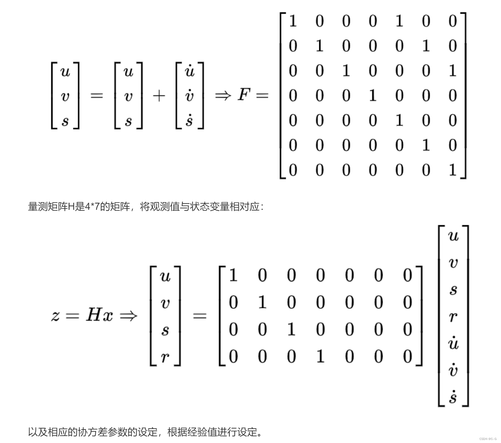
               [[1, 0, 0, 0, 1, 0, 0], [0, 1, 0, 0, 0, 1, 0], [0, 0, 1, 0, 0, 0, 1], [0, 0, 0, 1, 0, 0, 0],
                [0, 0, 0, 0, 1, 0, 0], [0, 0, 0, 0, 0, 1, 0], [0, 0, 0, 0, 0, 0, 1]])
           # H Is the measurement matrix , yes 4*7 Matrix 
           self.kf.H = np.array(
               [[1, 0, 0, 0, 0, 0, 0], [0, 1, 0, 0, 0, 0, 0], [0, 0, 1, 0, 0, 0, 0], [0, 0, 0, 1, 0, 0, 0]])
           # R Is the covariance of the measurement noise , That is, the covariance of the difference between the real value and the measured value 
           self.kf.R[2:, 2:] *= 10.
           # P Is the covariance of a priori estimate 
           self.kf.P[4:, 4:] *= 1000.  # give high uncertainty to the unobservable initial velocities
           self.kf.P *= 10.
           # Q Is the covariance of the process excitation noise 
           self.kf.Q[-1, -1] *= 0.01
           self.kf.Q[4:, 4:] *= 0.01
           #  State estimation 
           self.kf.x[:4] = convert_bbox_to_z(bbox)
           #  Parameter update 
           self.time_since_update = 0
           self.id = KalmanBoxTracker.count
           KalmanBoxTracker.count += 1
           self.history = []
           self.hits = 0
           self.hit_streak = 0
           self.age = 0

• Update state variables
  Update the state variable with the observed target box

 def update(self, bbox):
        #  Reset 
        self.time_since_update = 0
        #  Empty history
        self.history = []
        # hits Count plus 1
        self.hits += 1
        self.hit_streak += 1
        #  Modify the internal state according to the observation results x
        self.kf.update(convert_bbox_to_z(bbox))

• Forecast the target box
  Advance the state variable and return the predicted bounding box result

    def predict(self):
        #  Push state variables 
        if (self.kf.x[6] + self.kf.x[2]) <= 0:
            self.kf.x[6] *= 0.0
        #  To make predictions 
        self.kf.predict()
        #  The number of Kalman filters 
        self.age += 1
        #  If not updated during the process , take hit_streak Set as 0
        if self.time_since_update > 0:
            self.hit_streak = 0
        self.time_since_update += 1
        #  Append forecast results to history in 
        self.history.append(convert_x_to_bbox(self.kf.x))
        return self.history[-1]

• The overall code

class KalmanBoxTracker(object):
    count = 0

    def __init__(self, bbox):
        """  Initialize the bounding box and tracker  :param bbox: """
        #  Define the isokinetic model 
        #  For internal use KalmanFilter,7 State variables and 4 Observation inputs 
        self.kf = KalmanFilter(dim_x=7, dim_z=4)
        self.kf.F = np.array(
            [[1, 0, 0, 0, 1, 0, 0], [0, 1, 0, 0, 0, 1, 0], [0, 0, 1, 0, 0, 0, 1], [0, 0, 0, 1, 0, 0, 0],
             [0, 0, 0, 0, 1, 0, 0], [0, 0, 0, 0, 0, 1, 0], [0, 0, 0, 0, 0, 0, 1]])
        self.kf.H = np.array(
            [[1, 0, 0, 0, 0, 0, 0], [0, 1, 0, 0, 0, 0, 0], [0, 0, 1, 0, 0, 0, 0], [0, 0, 0, 1, 0, 0, 0]])
        self.kf.R[2:, 2:] *= 10.
        self.kf.P[4:, 4:] *= 1000.  # give high uncertainty to the unobservable initial velocities
        self.kf.P *= 10.
        self.kf.Q[-1, -1] *= 0.01
        self.kf.Q[4:, 4:] *= 0.01
        self.kf.x[:4] = convert_bbox_to_z(bbox)
        self.time_since_update = 0
        self.id = KalmanBoxTracker.count
        KalmanBoxTracker.count += 1
        self.history = []
        self.hits = 0
        self.hit_streak = 0
        self.age = 0

    def update(self, bbox):
        """  Update the state vector with the observed target box .filterpy.kalman.KalmanFilter.update  Internal state estimates will be modified based on observations self.kf.x.  Reset self.time_since_update, Empty self.history. :param bbox: Target box  :return: """
        self.time_since_update = 0
        self.history = []
        self.hits += 1
        self.hit_streak += 1
        self.kf.update(convert_bbox_to_z(bbox))

    def predict(self):
        """  Advance the state vector and return the predicted bounding box estimate .  Append forecast results to self.history. because  get_state  Direct access  self.kf.x, therefore self.history Not used  :return: """
        if (self.kf.x[6] + self.kf.x[2]) <= 0:
            self.kf.x[6] *= 0.0
        self.kf.predict()
        self.age += 1
        if self.time_since_update > 0:
            self.hit_streak = 0
        self.time_since_update += 1
        self.history.append(convert_x_to_bbox(self.kf.x))
        return self.history[-1]

    def get_state(self):
        """  Returns the current bounding box estimate  :return: """
        return convert_x_to_bbox(self.kf.x)

In Hungary, 、KM Algorithm

hungarian algorithm （Hungarian Algorithm） And KM Algorithm （Kuhn-Munkres Algorithm） It is used to solve the problem of data association in multi-target tracking , Hungarian algorithm and KM All the algorithms are to solve the maximum matching problem of bipartite graph .

There is a very special kind of graph , Just make a bipartite graph , What is a bipartite graph ？ Can be divided into two groups ,U,V. among ,U Points on cannot be connected to each other , We can only connect V In the point , Empathy ,V Points in cannot be connected to each other , We can only connect U In the point . such , It's called a bipartite graph .

The bipartite graph can be understood as all detection frames in two consecutive frames in the video , The set of all detection frames in the first frame is called U, The set of all detection frames in the second frame is called V. Different detection frames in the same frame will not be the same target , So there's no need to correlate , The detection frames of two adjacent frames need to be connected with each other , Finally, the detection frames of two adjacent frames are matched as perfectly as possible . The optimal solution to this problem requires the Hungarian algorithm or KM Algorithm .

hungarian algorithm

Hungarian algorithm is a combinatorial optimization algorithm to solve the task allocation problem in polynomial time . American mathematician Harold · Kuhn in 1955 The algorithm was proposed in . This algorithm is called Hungarian algorithm , It's because algorithms are largely based on former Hungarian mathematicians Dénes Kőnig and Jenő Egerváry Created on top of the work of .

We introduce the Hungarian algorithm with the method of target tracking , The following is an example , Let's assume that the four graphs on the left are us at N Frame detected target （U）, The four pictures on the right show us at number N+1 Frame detected target （V）. A picture with red lines , It's our algorithm that thinks it's a more likely target for the same pedestrian . Because the algorithm is not absolutely ideal , So it's not necessarily guaranteed that every graph has a one-to-one match , One to two or even one to many , Even many to many situations happen from time to time . How do we get the final one-on-one tracking results ？ Let's see how the Hungarian algorithm works .

• First step
  First, left 1 Match , Find the first right... Connected to it 1 Is not match , Pair it up , Connect a blue line .
  
• The second step
  Then match left 2, Find the first target connected to it right 2 Is not match , Pair it up
  
• The third step
  ** And then left 3, Find the top priority right 1 The match is done , What shall I do? ？

We give it to the right before 1 Match object left of 1 Assign another object .

（ Yellow means the edge has been temporarily removed ）**

** Can be with left 1 The second target of the match is right 2, But right 2 There are already matching objects , What shall I do? ？

Let's give it back to you 2 Match object left of 2 Assign another object （ Note that this step is the same as above , This is a recursive process ）.**

** At this point, we found that left 2 It can also match right 3, Then the previous problem is solved , Go back to .

Left 2 Right 3, Left 1 Right 2, Left 3 Right 1.**

So the final result of the third step is ：

Finally, left 4, unfortunately , According to the rhythm of step three, we can't give left 4 Free up a match , Can only give up on the left 4 The matching of , This is the end of the Hungarian algorithm . The blue line is our final match . So far, we have found a maximum match of this bipartite graph . The end result is that we match three pairs of targets , Because the candidate matching target contains many wrong matching red lines （ edge ）, So the matching accuracy is not high . It can be seen that Hungarian algorithm requires high accuracy of red line connection , That is to ask us to move the model 、 Parts such as appearance models must be predicted accurately , Or set a higher threshold , Only the edge with high confidence is sent to Hungary algorithm for matching , Only in this way can we get better results .

You can see the process of Hungarian algorithm , There is a very obvious problem, I believe you have also found , The biggest match found in this way is often not the best in our mind . The Hungarian algorithm considers the status of each matching object as the same , Under this premise, the maximum matching is solved . This is not in accordance with our multi-target tracking problem , Because every matching object can't be of equal status , There's always a real goal that is the best match we're looking for , And this real goal should have a higher weight , On this basis, the matching results can be closer to the real situation .

KM The algorithm can solve this problem better , Let's take a look KM Algorithm .

KM Algorithm

KM The algorithm solves the optimal matching problem of weighted bipartite graph .

Let's take the above figure as an example , This time, weight is added to each connection , That is, the confidence score given by other modules in our algorithm .

• First step
  First assign a value to each vertex , It is called the top mark , Assign the vertex on the left the maximum weight of the edge connected to it , The vertex on the right is assigned 0.
  
• The second step
  The matching principle is only with the weight and the score on the left （ Top mark ） Match the same edges , If no edge match is found , Subtract the top mark of all left vertices of this path d, Add... To the top of all right vertices d. Parameters d We take the value here as 0.1.

For left 1, The side with the same score as the top mark shall be marked with blue first .

Then left 2, The side mark with the same score as the top mark

Then left 3, Discovery and right 1 Already with left 1 pairing . First of all, I want to let Zuo 3 Replace the matching object , However, according to the matching principle , Only the weight is greater than or equal to 0.9+0=0.9（ Left top mark plus right top mark ） The edge of the can meet the requirements . So left 3 Cannot switch sides . That left 1 Can you change sides ？ For left 1 Come on , Only the weight is greater than or equal to 0.8+0=0.8 The edge of the can meet the requirements , Cannot switch sides . At this point, according to KM Algorithm , The vertices of all conflicting edges should be added or subtracted , Reduce the value of the left vertex by 0.1, The right vertex value plus 0.1. The results are shown in the following figure .

Then perform the matching operation , Found left 3 One more matching edge , Because at this time left 3 Right 2 The matching requirement of only needs the weight to be greater than or equal to 0.8+0 that will do , So left 3 And right 2 matching

Finally, proceed to the left 4 The matching of , Due to left 4 The only matching object right 3 Has been left 2 matching , conflict . Make a round of addition and subtraction d operation , Match again , The left four still failed to match . Two rounds later left 4 The expectation is reduced to 0, Discard matching left 4.

thus KM The algorithm flow ends , Three pairs of targets match successfully , Even when the prediction of the left three targets is not accurate enough, the correct matching is carried out . It can be seen that after the introduction of weight , The matching success rate is greatly improved ..

Finally, there is one more point worth noting , The maximum match obtained by Hungarian algorithm is not unique , Preset matching edges 、 Or the matching order is different , Can lead to multiple maximum matches , So there is an alternative KM The idea of the algorithm is , We just need to use Hungarian algorithm to find all the maximum matches , Compare the weights of each maximum match , Then select the optimal matching with the maximum weight to get the matching result closer to the real situation . But this method has high time complexity , As the number of goals increases , The time consumed is greatly increased , It is not recommended in practical use .

Implementation of Hungarian algorithm

scipy.optimize.linear_sum_assignment(cost_matrix)

Realization KM Algorithm , among const_matrix Represents the cost matrix . For example, the first frame has a,b,c,d Four goals , The second image has p,q,r,s Four goals , The similarity matrix is as follows ：

from scipy.optimize import linear_sum_assignment
import numpy as np
#  Cost matrix 
cost =np.array([[0.9,0.6,0,0],[0,0.3,0.9,0],[0.5,0.9,0,0],[0,0,0.2,0]])
#  Matching results ： The purpose of this method is to minimize the cost , Here is the maximum match , So will cost Take a negative number 
row_ind,col_ind=linear_sum_assignment(-cost)
# The corresponding row index 
print(" Row index ：\n{}".format(row_ind))
# The best assigned column index for the row index 
print(" Column index ：\n{}".format(col_ind))
# Extract the optimal index of each row index to the element where the index is located , Form an array 
print(" Matching degree ：\n{}".format(cost[row_ind,col_ind]))

Data Association

Here we match the detection box with the tracking box , The whole process is to traverse the detection box and the tracking box , And match , If the match succeeds, keep it , Failed to delete it .

def associate_detections_to_trackers(detections, trackers, iou_threshold=0.3):
    """  The detection box bbox And the tracking frame of the Kalman filter  :param detections: Check box  :param trackers: Tracking box , That is, tracking the target  :param iou_threshold:IOU threshold  :return: A matrix for tracking success goals ：matchs  Matrix of new targets ：unmatched_detections  If the tracking fails, it will leave the target matrix of the screen ：unmatched_trackers """
    #  The number of tracking targets is 0, Direct construction results 
    if (len(trackers) == 0) or (len(detections) == 0):
        return np.empty((0, 2), dtype=int), np.arange(len(detections)), np.empty((0, 5), dtype=int)

    # iou  Array calculation is not supported . Calculate the intersection and union ratio of two pairs one by one , call  linear_assignment  Match 
    iou_matrix = np.zeros((len(detections), len(trackers)), dtype=np.float32)
    #  Traverse the target detection bbox aggregate , The identification of each detection box is d
    for d, det in enumerate(detections):
        #  Traverse the trace box （ Kalman filter prediction ）bbox aggregate , Each trace box is identified as t
        for t, trk in enumerate(trackers):
            iou_matrix[d, t] = iou(det, trk)
    #  The tracking frame and the detection frame are separated by the Hungarian algorithm [[d,t]...] The form of a two-dimensional matrix is stored in match_indices in 
    result = linear_sum_assignment(-iou_matrix)
    matched_indices = np.array(list(zip(*result)))

    #  Record the unmatched detection box and tracking box 
    #  Unmatched detection boxes are placed in unmatched_detections in , Indicates that a new target has entered the screen , To add a tracker to track the target 
    unmatched_detections = []
    for d, det in enumerate(detections):
        if d not in matched_indices[:, 0]:
            unmatched_detections.append(d)
    #  Unmatched trace boxes are placed in unmatched_trackers in , Indicates the picture before the target leaves , The corresponding tracker should be deleted 
    unmatched_trackers = []
    for t, trk in enumerate(trackers):
        if t not in matched_indices[:, 1]:
            unmatched_trackers.append(t)
    #  Put the successfully matched trace box into matches in 
    matches = []
    for m in matched_indices:
        #  To filter out IOU Low matching , Put it in unmatched_detections and unmatched_trackers
        if iou_matrix[m[0], m[1]] < iou_threshold:
            unmatched_detections.append(m[0])
            unmatched_trackers.append(m[1])
        #  If the conditions are met, take [[d,t]...] In the form of matches in 
        else:
            matches.append(m.reshape(1, 2))
    #  initialization matches, With np.array Form return of 
    if len(matches) == 0:
        matches = np.empty((0, 2), dtype=int)
    else:
        matches = np.concatenate(matches, axis=0)

    return matches, np.array(unmatched_detections), np.array(unmatched_trackers)

SORT/deepSORT

SORT and DeepSORT It is two well-known algorithms in multi-target tracking .DeepSORT It is the original team that is right SORT Improved version .

SORT

SORT The core is Kalman filter and Hungarian matching algorithm . The flow chart is shown below , You can see that the whole can be divided into two parts , They are the matching process and the Kalman prediction plus update process , It's all marked in gray boxes .

Key steps ： Trajectory Kalman filter prediction → The Hungarian algorithm is used to predict the tracks And... In the current frame detecions Match （IOU matching ） → Kalman filter update

Kalman filter is divided into two processes ： Forecast and update .SORT Linear velocity model and Kalman filter are introduced to predict the position , First make location prediction, and then match . The results of the motion model can be used to predict the position of the object .

The Hungarian algorithm solves an assignment problem , use IOU Distance as weight （ Also called cost matrix ）, And when the IOU Less than a certain value , Don't think it's the same goal , The theoretical basis is that the object in the video will not move too much between two frames . The threshold selected in the code is 0.3.scipy Library linear_sum_assignment Have implemented this algorithm , Just input cost_matrix That is, the cost matrix can get the best match .

DeepSort

DeepSORT yes SORT Sequels , There is no big change in the overall framework , Or continue the idea of Kalman filter plus Hungary algorithm , On this basis, the authentication network is added Deep Association Metric.

The picture below is deepSORT flow chart , and SORT Is essentially the same , There's more cascade matching （Matching Cascade） And the confirmation of the new track （confirmed）.

Key steps ： Trajectory Kalman filter prediction → The Hungarian algorithm is used to predict the tracks And... In the current frame detecions Match （ Cascade matching and IOU matching ） → Kalman filter update

The cascade matching flow chart is as follows ：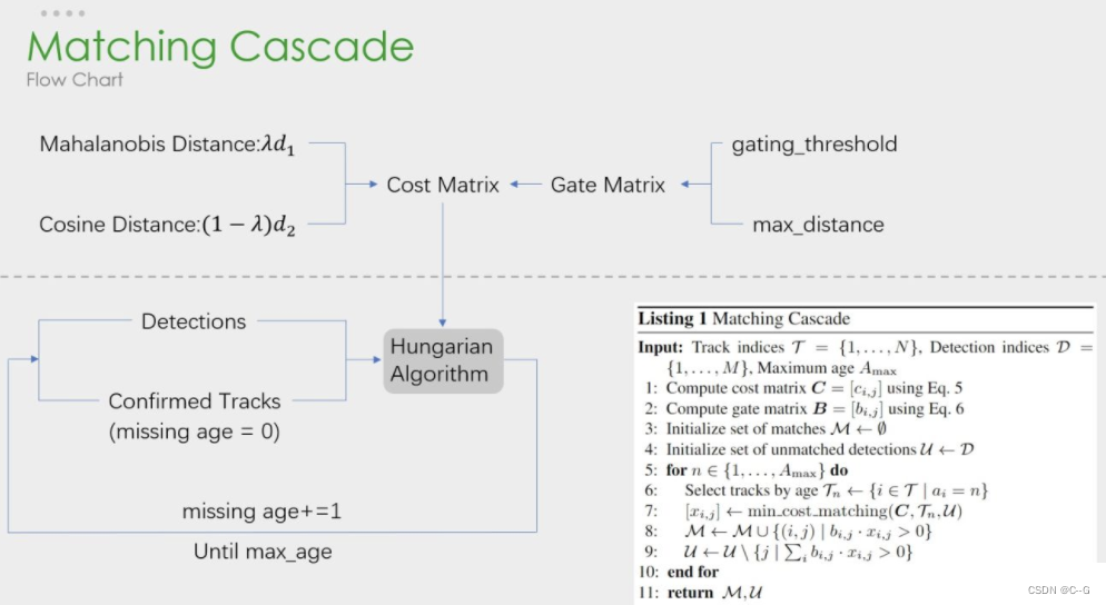

The first half is the similarity estimation , That is to calculate the cost function of this allocation problem . In the second half, the Hungarian algorithm is still used to match the detection frame and the tracking frame .

Multi target tracking

Here we mainly implement a multi-target tracker , Manage multiple Kalman filter objects , It mainly includes the following contents ：

initialization ： Maximum number of detections , The maximum number of frames the target is not detected
Update of target tracking results , That is, tracking the updates of successful and failed targets

• initialization

 def __init__(self, max_age=1, min_hits=3):
        """  initialization ： Set up SORT Key parameters of the algorithm  """
        #  Maximum number of detections ： Number of frames in which the target has not been detected , After that, it will be deleted  
        self.max_age = max_age
        #  The minimum number of target hits , If it is less than this number, it will not return 
        self.min_hits = min_hits  
        #  Kalman tracker 
        self.trackers = []  
        #  Frame count 
        self.frame_count = 0

• Update of target tracking results
  This method implements SORT Algorithm , Input is a collection of detection boxes for all objects in the current frame , Including the target score, The output is the set of tracking frames of the current frame , Including target tracking id The requirement is that even if the detection box is empty , This method must also be called for each frame , Returns a similar output array , The last column is the target object id. It should be noted that , The number of returned target objects may be different from the number of detection boxes .
  

    def update(self, dets):
        self.frame_count += 1
        #  Predict track positions one by one at the current frame , Tracker index for logging status exceptions 
        #  According to the current number of all Kalman trackers （ That is, the number of targets tracked in the previous frame ） Create a 2D array ： The line number is the identification index of Kalman filter , The column vector is the position of the tracking box and ID
        trks = np.zeros((len(self.trackers), 5))  #  Store tracker predictions 
        to_del = []   #  Store the target box to delete 
        ret = []    #  Store the tracking target box to return 
        #  Loop through the Kalman tracker list 
        for t, trk in enumerate(trks):
            #  Using the Kalman tracker t Generate a tracking frame corresponding to the target 
            pos = self.trackers[t].predict()[0]
            #  After traversal ,trk The prediction tracking frame of the target tracked in the previous frame is stored in 
            trk[:] = [pos[0], pos[1], pos[2], pos[3], 0]
            #  If the tracking box contains a null value, add the tracking box to the list to be deleted 
            if np.any(np.isnan(pos)):
                to_del.append(t)
        # numpy.ma.masked_invalid  Mask arrays with invalid values （NaN  or  inf）
        # numpy.ma.compress_rows  Compress the with mask values 2-D  The entire row of the array , Remove the entire line containing the mask value 
        # trks A prediction tracking frame in which the target tracked in the previous frame and in the current frame are stored 
        trks = np.ma.compress_rows(np.ma.masked_invalid(trks))
        #  Reverse delete exception tracker , Prevent index corruption 
        for t in reversed(to_del):
            self.trackers.pop(t)
        #  The target detection frame is associated with the tracking frame predicted by the Kalman filter to obtain the successfully tracked target , New target , Leave the target of the picture 
        matched, unmatched_dets, unmatched_trks = associate_detections_to_trackers(dets, trks)

        #  Update the tracking successful target frame to the corresponding Kalman filter 
        for t, trk in enumerate(self.trackers):
            if t not in unmatched_trks:
                d = matched[np.where(matched[:, 1] == t)[0], 0]
                #  Update the state vector with the observed bounding box 
                trk.update(dets[d, :][0])

        #  Create a new Kalman filter object to track the new target 
        for i in unmatched_dets:
            trk = KalmanBoxTracker(dets[i, :])
            self.trackers.append(trk)

        #  Traverse backwards and forwards , Return only if it occurs in the current frame and the hit period is greater than self.min_hits（ Unless the tracking just started ） Tracking results for ; If the miss time is greater than self.max_age Then delete the tracker .
        # hit_streak Ignore the initial frames of the target 
        i = len(self.trackers)
        for trk in reversed(self.trackers):
            #  Returns the estimated value of the current bounding box 
            d = trk.get_state()[0]
            #  Track success goals box And id Put in ret In the list 
            if (trk.time_since_update < 1) and (trk.hit_streak >= self.min_hits or self.frame_count <= self.min_hits):
                ret.append(np.concatenate((d, [trk.id + 1])).reshape(1, -1))  # +1 as MOT benchmark requires positive
            i -= 1
            #  The target that fails to track or leaves the picture is deleted from the Kalman tracker 
            if trk.time_since_update > self.max_age:
                self.trackers.pop(i)
        #  Return to... Of all targets in the current screen box And id, Returns... As a two-dimensional matrix 
        if len(ret) > 0:
            return np.concatenate(ret)
        return np.empty((0, 5))

yoloV3 Model

yoloV3 With V1,V2 Improvements based on , There are mainly ： Target detection using multi-scale features ; A priori boxes are richer ; Adjusted the network structure ; Object classification uses logistic Instead of softmax, It is more suitable for multi label classification tasks .

Introduction to the algorithm

YOLOv3 yes YOLO (You Only Look Once) Series of target detection algorithm in the third edition , Compared with the previous algorithm , Especially for small targets , The accuracy has been significantly improved .

yoloV3 The process is shown in the figure below , For each input image ,YOLOv3 Will predict the output of three different scales , The purpose is to detect targets of different sizes .

Multiscale detection

Usually an image contains a variety of different objects , And there are big and small . Ideally, objects of all sizes can be detected at the same time . therefore , The network must be able to “ notice ” The ability of objects of different sizes . Because the deeper the network , The smaller the feature map , So the deeper the network, the harder it is to detect small objects .

In practice feature map in , With the deepening of network depth , Shallow feature map It mainly contains low-level information （ The edge of the object , Color , Primary location information, etc ）, Deep feature map Contains advanced information （ For example, the semantic information of objects ： Dog , cat , Cars, etc. ）. So at different levels feature map Corresponding to different scale, Therefore, we can detect targets in different levels of feature maps . The following figure shows a variety of scale Classical method of transformation .

(a) This method first establishes the image pyramid , Pyramid images of different scales are input into the corresponding network , For different scale Object detection . But the result is that each level of pyramid needs to be processed once , slowly , stay SPPNet That's how it works .

(b) The detection is only on the last layer feature map Phase in , This structure cannot detect objects of different sizes

For different depths feature map Target detection respectively .SSD Such a structure is adopted in . Such a small object will be in the shallow feature map Detected in , And large objects will be in the deep feature map Detected , So as to correspond to different scale The purpose of the object , The disadvantage is that every feature map The information obtained only comes from the previous layer , The characteristic information of the subsequent layer cannot be obtained and used .

(d) Very close to , But the difference is , Current layer's feature map For the future feature map Sample up , And make use of . Because of such a structure , Current feature map You can get “ future ” Layer information , In this way, low-order features and high-order features are organically integrated , Improve the detection accuracy . stay YOLOv3 in , This is the way to realize the multi-scale transformation of the target .

Network model structure

In the basic image feature extraction ,YOLO3 Adopted Darknet-53 Network structure （ contain 53 Convolution layers ）, It draws on the residual network ResNet How to do it , Between the layers shortcut, To solve the problem of deep network gradient ,shortcut As shown in the figure below ： It contains two convolution layers and one shortcut connections.

yoloV3 The structure of the model is as follows

Whole v3 Inside the structure , There is no pooling layer and full connectivity layer , The down sampling of the network is achieved by setting convolution stride by 2 To achieve , Every time you pass through this convolution, the size of the image is reduced to half . In the residual module 1×,2×,8×,8× Etc. indicates the number of residual modules .

A priori box

yoloV3 use K-means The size of a priori frame is obtained by clustering , Set... For each scale 3 A priori frame , A total of 9 A priori frame of two sizes .

stay COCO The dataset is 9 A priori box is ：(10x13),(16x30),(33x23),(30x61),(62x45),(59x119),(116x90),(156x198),(373x326). In the smallest (13x13) On the characteristic map （ Have the greatest feeling field ） Apply a larger a priori box (116x90),(156x198),(373x326), Suitable for detecting large objects . medium (26x26) On the characteristic map （ Medium receptive field ） Apply medium a priori box (30x61),(62x45),(59x119), Suitable for detecting medium-sized objects . The larger (52x52) On the characteristic map （ Smaller receptive fields ） application , The smaller a priori box (10x13),(16x30),(33x23), Suitable for detecting smaller objects .

Intuitively feel 9 The size of a priori box , The blue box in the figure below is the prior box obtained by clustering . Yellow frame ground truth, The red box is the grid where the center point of the object is located .

ligistic Return to

Do not use... When predicting object categories softmax, Instead, it is replaced by a 1x1 The convolution of layer +logistic The structure of the activation function . Use softmax In fact, it has been assumed that each output only corresponds to a single class, But in some class There is overlap （ for example woman and person） Data set , Use softmax Can't make the network predict the data well .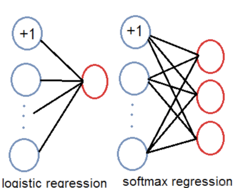

yoloV3 The input and output of the model

YoloV3 The input and output form of is shown in the figure below

Input 416×416×3 Image , adopt darknet The network obtains the prediction results of three different scales , Each scale corresponds to N Channels , Contains predictive information ;

Of each grid and size anchors Forecast results of .

YOLOv3 share 13×13×3 + 26×26×3 + 52×52×3 Forecast . Each prediction corresponds to 85 dimension , Namely 4（ Coordinate value ）、1（ Confidence score ）、80（coco Category probability ）.

be based on yoloV3 Target detection for

The object detection we performed here is based on OPenCV The use of yoloV3 Target detection , Don't involve yoloV3 Model structure of 、 Theory and training process , Just use the trained model for target detection

• load yolov3 Model and its weight parameters

# 1. Load a name that identifies the object , Store it LABELS in , Altogether 80 Kind of , Here we only use car
labelsPath = "./yolo-coco/coco.names"
LABELS = open(labelsPath).read().strip().split("\n")

#  Set random number seed , Generate many different colors , When there are multiple targets in a picture , Frame it with boxes of different colors 
np.random.seed(42)
COLORS = np.random.randint(0, 255, size=(200, 3),dtype="uint8")

#  Load trained yolov3 The weight of the network and the corresponding configuration data 
weightsPath = "./yolo-coco/yolov3.weights"
configPath = "./yolo-coco/yolov3.cfg"

#  After loading the data , Start using the above data to recover yolo neural network 
net = cv2.dnn.readNetFromDarknet(configPath, weightsPath)
#  obtain YOLO The name of each network layer in ：['conv_0', 'bn_0', 'relu_0', 'conv_1', 'bn_1', 'relu_1', 'conv_2', 'bn_2', 'relu_2'...]
ln = net.getLayerNames()
#  Get the index position of the output layer in the network , And in the form of a list ：['yolo_82', 'yolo_94', 'yolo_106']
ln = [ln[i[0] - 1] for i in net.getUnconnectedOutLayers()]

• The image to be processed is converted into the blobs

# 2.  Read images 
frame = cv2.imread("./images/car1.jpg")
#  The width and height of the video , Frame size 
(W, H) = (None, None)
if W is None or H is None:
    (H, W) = frame.shape[:2]

#  Construct according to the input image blob, utilize OPenCV When calculating the depth network , Generally, the image is converted to blob form , Preprocess the picture , Including zoom , Minus mean , Channel switching, etc 
#  You can also set the size , It is generally set to the size of the image during network training 
blob = cv2.dnn.blobFromImage(frame, 1 / 255.0, (416, 416), swapRB=True, crop=False)

• Use the model to detect the target

# 3. take blob Input into the forward network , And make predictions 
net.setInput(blob)
start = time.time()
# yolo Feedforward calculation , Get the boundary and the corresponding probability 
#  Output layerOutsputs Introduce ：
#  yes YOLO Algorithm detected in the picture bbx Information about 
#  because YOLO v3 There are three outputs , That's what I mentioned above ['yolo_82', 'yolo_94', 'yolo_106']
#  therefore layerOutsputs Is a length of 3 A list of 
#  among , The dimension of each element in the list is (num_detection, 85)
# num_detections Indicates that the output of this layer has detected bbx The number of 
# 85： Because the model is in COCO Training on data sets ,[5:] Indicates category probability ;[0:4] Express bbx Location information for ;[5] It means confidence 
layerOutputs = net.forward(ln)

• Traverse the detection results , Get the detection box

#  The following is about the network output bbx Inspection ：
#  Determine each bbx Whether the confidence level of is high enough , And perform NMS The algorithm removes redundant bbx

boxes = []  #  The information used to store the box identifying the object , Include the abscissa of the top left corner of the box x And the vertical y And the height of the frame h And width w
confidences = []  #  It indicates that the recognition target is a certain object 
classIDs = []  #  Indicates which category the identified target belongs to ,['person', 'bicycle', 'car', 'motorbike'....]

# 4.  Traverse the output of each output layer 
for output in layerOutputs:
    #  Traverse each target in an output layer 
    for detection in output:
        scores = detection[5:]  #  The probability that the current target belongs to a certain category 

        classID = np.argmax(scores)  #  Category of target ID
        confidence = scores[classID]  #  Get the confidence that the target belongs to this category 

        #  Only the retention reliability is greater than 0.3 The bounding box of , If the picture quality is poor , You can lower your confidence a little 
        if confidence > 0.3:
            #  Restore the coordinates of the bounding box to match the original picture ,YOLO Returns the center coordinates of the bounding box and the width and height of the bounding box 
            box = detection[0:4] * np.array([W, H, W, H])
            (centerX, centerY, width, height) = box.astype("int") #  Use  astype("int")  For the above  array  Cast ,centerX： Abscissa of the center point of the frame , centerY： Vertical coordinate of the center point of the frame ,width： The width of the frame ,height： The height of the frame 

            x = int(centerX - (width / 2))  #  Calculate the abscissa of the upper left corner of the bounding box 
            y = int(centerY - (height / 2))  #  Calculate the vertical coordinate of the upper left corner of the bounding box 

            #  Update the detected target box , Confidence and category ID
            boxes.append([x, y, int(width), int(height)])  #  Add border information to the list boxes
            confidences.append(float(confidence))  #  Add the confidence level to the list that the object is recognized confidences
            classIDs.append(classID) #  Add to the list information that identifies which class the object belongs to classIDs

• Non maximum suppression

# 5.  Non maximum suppression 
idxs = cv2.dnn.NMSBoxes(boxes, confidences, 0.5, 0.3)

• Final test results , draw , And deposit it in ndarray in , For target tracking

# 6.  Get the final test results 
dets = []  #  Store the information of the detection box , Including the abscissa of the upper left corner , Ordinate , Abscissa in the lower right corner , Ordinate , And the confidence of the detected object , For target tracking 
if len(idxs) > 0:  #  If there is a detection box （ That is, the number of detection frames is greater than 0）
    for i in idxs.flatten():  #  Loop through each detected box
        # yolo The model can identify many targets , Because we are here just to identify the car , So only if the target is a car, we will test it , Other neglect 
        if LABELS[classIDs[i]] == "car":
            (x, y) = (boxes[i][0], boxes[i][1])  #  Get the coordinates of the upper left corner of the detection box 
            (w, h) = (boxes[i][2], boxes[i][3])  #  Get the width and height of the detection frame 
            cv2.rectangle(frame, (x, y), (x+w, y+h), (0,255,0), 2)  #  Draw the box on the screen 
            dets.append([x, y, x + w, y + h, confidences[i]])  #  Put the information of the detection box into dets in 
#  Set data type , Convert integer data to floating point number type , And keep three decimal places 
np.set_printoptions(formatter={
    'float': lambda x: "{0:0.3f}".format(x)})
#  Convert the detection frame data to ndarray, Its data type is floating point type 
dets = np.asarray(dets)

plt.imshow(frame[:,:,::-1])

• Object detection in video

labelsPath = "./yolo-coco/coco.names"
LABELS = open(labelsPath).read().strip().split("\n")

#  Set random number seed , Generate many different colors , When there are multiple targets in a picture , Frame it with boxes of different colors 
np.random.seed(42)
COLORS = np.random.randint(0, 255, size=(200, 3),dtype="uint8")

#  Load trained yolov3 The weight of the network and the corresponding configuration data 
weightsPath = "./yolo-coco/yolov3.weights"
configPath = "./yolo-coco/yolov3.cfg"

#  After loading the data , Start using the above data to recover yolo neural network 
net = cv2.dnn.readNetFromDarknet(configPath, weightsPath)
#  obtain YOLO The name of each network layer in ：['conv_0', 'bn_0', 'relu_0', 'conv_1', 'bn_1', 'relu_1', 'conv_2', 'bn_2', 'relu_2'...]
ln = net.getLayerNames()
#  Get the index position of the output layer in the network , And in the form of a list ：['yolo_82', 'yolo_94', 'yolo_106']
ln = [ln[i[0] - 1] for i in net.getUnconnectedOutLayers()]

"""  Video processing class  """

#  initialization vediocapture class , Parameter specifies the open video file , It can also be a camera 
vs = cv2.VideoCapture('./input/test_1.mp4')
#  The width and height of the video , Frame size 
(W, H) = (None, None)
#  Video file write object 
writer = None

try:
    #  Determine how to get the number of video frames 
    prop = cv2.cv.CV_CAP_PROP_FRAME_COUNT if imutils.is_cv2() \
        else cv2.CAP_PROP_FRAME_COUNT
    #  Get the total number of frames of the video 
    total = int(vs.get(prop))
    #  Number of frames to print video 
    print("[INFO] {} total frames in video".format(total))
except:
    print("[INFO] could not determine # of frames in video")
    print("[INFO] no approx. completion time can be provided")
    total = -1

#  Cycle through each frame of the video 
while True:
    #  Read frame ：grabbed yes bool, Indicates whether the frame was captured successfully ,frame Is the captured frame 
    (grabbed, frame) = vs.read()
    #  If no frame is captured , Then exit the loop 
    if not grabbed:
        break
    #  if W and H It's empty , Then assign the size of the first frame to him 
    if W is None or H is None:
        (H, W) = frame.shape[:2]

    #  Construct according to the input image blob, utilize OPenCV When calculating the depth network , Generally, the image is converted to blob form , Preprocess the picture , Including zoom , Minus mean , Channel switching, etc 
    #  You can also set the size , It is generally set to the size of the image during network training 
    blob = cv2.dnn.blobFromImage(frame, 1 / 255.0, (416, 416), swapRB=True, crop=False)
    #  take blob Input into the forward network 
    net.setInput(blob)
    start = time.time()
    # yolo Feedforward calculation , Get the boundary and the corresponding probability 
    layerOutputs = net.forward(ln)
    """  Output layerOutsputs Introduce ：  yes YOLO Algorithm detected in the picture bbx Information about   because YOLO v3 There are three outputs , That's what I mentioned above ['yolo_82', 'yolo_94', 'yolo_106']  therefore layerOutsputs Is a length of 3 A list of   among , The dimension of each element in the list is (num_detection, 85) num_detections Indicates that the output of this layer has detected bbx The number of  85： Because the model is in COCO Training on data sets ,[5:] Indicates category probability ;[0:4] Express bbx Location information for ;[5] It means confidence  """
    end = time.time()

    """  The following is about the network output bbx Inspection ：  Determine each bbx Whether the confidence level of is high enough , And perform NMS The algorithm removes redundant bbx """
    boxes = []  #  The information used to store the box identifying the object , Include the abscissa of the top left corner of the box x And the vertical y And the height of the frame h And width w
    confidences = []  #  It indicates that the recognition target is a certain object 
    classIDs = []  #  Indicates which category the identified target belongs to ,['person', 'bicycle', 'car', 'motorbike'....]

    #  Traverse the output of each output layer 
    for output in layerOutputs:
        #  Traverse each target in an output layer 
        for detection in output:
            scores = detection[5:]  #  The probability that the current target belongs to a certain category 
            """ # scores = detection[5:] ---> [0. 0. 0. 0. 0. 0. 0. 0. 0. 0. 0. 0. 0. 0. 0. 0. 0. 0. 0. 0. 0. 0. 0. 0. # 0. 0. 0. 0. 0. 0. 0. 0. 0. 0. 0. 0. 0. 0. 0. 0. 0. 0. 0. 0. 0. 0. 0. 0. # 0. 0. 0. 0. 0. 0. 0. 0. 0. 0. 0. 0. 0. 0. 0. 0. 0. 0. 0. 0. 0. 0. 0. 0. # 0. 0. 0. 0. 0. 0. 0. 0.] # scores The size of the should be 1*80, Because I'm training yolo The model is 80 Class target  """
            classID = np.argmax(scores)  #  Category of target ID
            confidence = scores[classID]  #  Get the confidence that the target belongs to this category 

            #  Only the retention reliability is greater than 0.3 The bounding box of , If the picture quality is poor , You can lower your confidence a little 
            if confidence > 0.3:
                #  Restore the coordinates of the bounding box to match the original picture ,YOLO Returns the center coordinates of the bounding box and the width and height of the bounding box 
                box = detection[0:4] * np.array([W, H, W, H])
                (centerX, centerY, width, height) = box.astype("int") #  Use  astype("int")  For the above  array  Cast ,centerX： Abscissa of the center point of the frame , centerY： Vertical coordinate of the center point of the frame ,width： The width of the frame ,height： The height of the frame 

                x = int(centerX - (width / 2))  #  Calculate the abscissa of the upper left corner of the bounding box 
                y = int(centerY - (height / 2))  #  Calculate the vertical coordinate of the upper left corner of the bounding box 

                #  Update the detected target box , Confidence and category ID
                boxes.append([x, y, int(width), int(height)])  #  Add border information to the list boxes
                confidences.append(float(confidence))  #  Add the confidence level to the list that the object is recognized confidences
                classIDs.append(classID) #  Add to the list information that identifies which class the object belongs to classIDs

    #  In the previous step, we have obtained yolo The detection frame of , But there will be redundancy bbox, That is, one target corresponds to multiple detection frames , So use NMS Remove duplicate detection boxes 
    #  utilize OpenCV Built in NMS DNN Module implementation can achieve non maximum suppression  , The required parameter is the boundary   box 、  Degree of confidence 、 And confidence thresholds and NMS threshold 
    #  The first parameter is the list of bounding boxes , The second parameter is the list of placement reliability , The third parameter is the confidence level you set , The fourth parameter is about threshold（ threshold 
    #  Back to idxs It's a one-dimensional array , The elements in the array are the remaining check boxes boxes Index position of 
    idxs = cv2.dnn.NMSBoxes(boxes, confidences, 0.5, 0.3)

    dets = []  #  Store the information of the detection box , Including the abscissa of the upper left corner , Ordinate , Abscissa in the lower right corner , Ordinate , And the confidence of the detected object , For target tracking 
    if len(idxs) > 0:  #  If there is a detection box （ That is, the number of detection frames is greater than 0）
        for i in idxs.flatten():  #  Loop through each detected box
            # yolo The model can identify many targets , Because we are here just to identify the car , So only if the target is a car, we will test it , Other neglect 
            if LABELS[classIDs[i]] == "car":
                (x, y) = (boxes[i][0], boxes[i][1])  #  Get the coordinates of the upper left corner of the detection box 
                (w, h) = (boxes[i][2], boxes[i][3])  #  Get the width and height of the detection frame 
                dets.append([x, y, x + w, y + h, confidences[i]])  #  Put the information of the detection box into dets in 
    #  Set data type , Convert integer data to floating point number type , And keep three decimal places 
    np.set_printoptions(formatter={
    'float': lambda x: "{0:0.3f}".format(x)})
    #  Convert the detection frame data to ndarray, Its data type is floating point type 
    dets = np.asarray(dets)

Traffic statistics

Vehicle statistics based on virtual coil method

The principle of traffic flow statistics algorithm based on virtual loop is similar to the common traditional physical loop on the traffic road , Because the physical coil needs to be buried under the road , Therefore, there will be installation 、 Maintenance costs are high , Cause pavement damage and other problems , The vehicle counting method based on video virtual coil completely avoids the above problems , And it can detect multiple regions of interest .

The principle of virtual loop vehicle counting method is in the collected traffic flow video , One or more detection lines shall be set on the road or section where vehicle counting is required to detect passing vehicles , So as to complete the counting work . The setting principle of detection line is generally to set a line perpendicular to the lane on the detection lane , Centered virtual line segment , By judging the change of its relative position to the passing vehicle , Complete the traffic flow statistics . As shown in the figure below , The green line is the virtual detection line ：

In this project, our testing method is , Calculate the central point line of the vehicle detection frame of the front and rear images , If the line intersects with the detection line , Then add one to the count , Otherwise, the count does not change .

How to judge whether two line segments intersect ？

Suppose there are two line segments AB,CD, if AB,CD The intersection , We can be sure ：

1. Line segment AB And CD Where the lines intersect , Immediate point A Sum point B In a straight line CD On both sides of ;

2. Line segment CD And AB Where the lines intersect , Immediate point C Sum point D In a straight line AB On both sides of ;

If the above two conditions are satisfied at the same time, it is a necessary and sufficient condition for the intersection of two segments , So we just need to prove something A Sum point B In a straight line CD On both sides of , spot C Sum point D In a straight line AB On both sides of , This proves that the line segment AB And CD Intersect .

In the diagram above , Line segment AB And line segments CD The intersection , So we can get two vectors AC,AD,C and D Respectively in AB On both sides of , vector AC In vector AB In the counter clockwise direction of ,AB×AC > 0; vector AD In vector AB In a clockwise direction ,AB×AD < 0, Two cross multiplication results in different sign .

such , The method comes out ： If the line segment CD Two endpoints of C and D, And an endpoint of another line segment （A or B, Only one of them ） Connected vectors , And vector AB Do cross product , If the result is different , Express C and D In a straight line AB On both sides of , If the result is the same , said CD At two o'clock AB One side of , It must not intersect .

So we use the cross ride method to judge whether the vehicle passes the detection line .

Realization

• testing AB and CD Whether the two lines intersect

#  testing AB and CD Whether the two lines intersect 
def intersect(A, B, C, D):
    return ccw(A, C, D) != ccw(B, C, D) and ccw(A, B, C) != ccw(A, B, D)

#  The calculation has A,B,C A vector of three points CA,BA The relationship between ,
def ccw(A, B, C):
    return (C[1] - A[1]) * (B[0] - A[0]) > (B[1] - A[1]) * (C[0] - A[0])

• Traverse the tracking box to determine whether it intersects with the detection line , And count the vehicles

#  Traverse the trace box 
for box in boxes:
    (x, y) = (int(box[0]), int(box[1]))  #  Calculate the coordinates of the upper left corner of the tracking box 
    (w, h) = (int(box[2]), int(box[3]))  #  Calculate the width and height of the tracking frame 

    color = [int(c) for c in COLORS[indexIDs[i] % len(COLORS)]]  #  Set the color of the box 
    cv2.rectangle(frame, (x, y), (w, h), color, 2)  #  Draw the box on the screen 

    """  According to the detection result of the current frame , It is connected with the detection of the previous frame , Carry out virtual coil to complete vehicle counting ： Traffic statistics  """
    if indexIDs[i] in previous:
        previous_box = previous[indexIDs[i]]  #  Get the target frame recognized in the previous frame 
        (x2, y2) = (int(previous_box[0]), int(previous_box[1]))  #  Get the coordinates of the upper left corner of the tracking frame of the previous frame 
        (w2, h2) = (int(previous_box[2]), int(previous_box[3]))  #  Obtain the width and height of the tracking frame of the previous frame 
        p0 = (int(x + (w - x) / 2), int(y + (h - y) / 2))  #  Get the center point of the current frame detection frame 
        p1 = (int(x2 + (w2 - x2) / 2), int(y2 + (h2 - y2) / 2))  #  Get the center point of the detection frame of the previous frame 
        cv2.line(frame, p0, p1, color, 3)  #  Connect the centers of the detection results of the two frames 

        """  Collision detection - The connecting line of the center point of the detection frame in the front and back frames crosses the reference line , Then count  """
        if intersect(p0, p1, line[0], line[1]):
            #  Total count plus 1
            counter += 1
            #  Judge the direction of travel 
            if y2 < y:
                counter_down += 1  #  Driving in reverse +1
            else:
                counter_up += 1  #  Driving in a positive direction +1

Traffic flow statistics in the video

We have completed the vehicle detection function in the video , Let's track the vehicle , And draw the tracking results in the video

• Track the target

    # yolo The test result in is 0 when , An error will appear in the incoming tracker , Judge here , No target tracking when no target is detected 
    if np.size(dets) == 0:
        continue
    else:
        tracks = tracker.update(dets)  #  Send the test results to the tracker , Return to the target successfully tracked in the current screen , Contains five messages ： Horizontal and vertical coordinates of the upper left and lower right corners of the target box , Confidence in the goal 

    #  Process the results returned by the tracker 
    boxes = []  #  Deposit tracks The first four values in ： The horizontal and vertical coordinates of the upper left corner and the horizontal and vertical coordinates of the lower right corner of the target box 
    indexIDs = []  #  Deposit tracks The last value in ： Degree of confidence , Used as a memory In the trace box Key
    previous = memory.copy()  #  Used to store the tracking results of the previous frame , For collision detection 
    memory = {
    } #  Store the tracking results of the target in the current frame , For collision detection 
    #  Traverse the trace results , Update the parameters 
    for track in tracks:
        boxes.append([track[0], track[1], track[2], track[3]])  #  Update the target frame coordinate information 
        indexIDs.append(int(track[4]))  #  Update confidence information 
        memory[indexIDs[-1]] = boxes[-1]  #  Place the trace box in key by ： Degree of confidence ,value by ： The tracking frame coordinates are stored in memory in 

• Draw information about the vehicle count

cv2.line(frame, line[0], line[1], (0, 255, 0), 3)  #  Draw it on the screen according to the set reference line 
cv2.putText(frame, str(counter), (30, 80), cv2.FONT_HERSHEY_DUPLEX, 3.0, (255, 0, 0), 3)  #  Plot the total count of vehicles 
cv2.putText(frame, str(counter_up), (130, 80), cv2.FONT_HERSHEY_DUPLEX, 3.0, (0, 255, 0), 3)  #  Draw the count of the vehicle moving in the forward direction 
cv2.putText(frame, str(counter_down), (230, 80), cv2.FONT_HERSHEY_DUPLEX, 3.0, (0, 0, 255), 3)  #  Plot the count of vehicles traveling in reverse 

• Save the results in the video

#  When the encoding and decoding information of the video is not set , Execute the following code 
    if writer is None:
        #  Set the encoding format 
        fourcc = cv2.VideoWriter_fourcc(*"mp4v")
        #  Video information settings 
        writer = cv2.VideoWriter("./output/output.mp4",
                                 fourcc,
                                 30,
                                 (frame.shape[1], frame.shape[0]),
                                 True)
    #  Write the processed frame to the video 
    writer.write(frame)
    #  Displays the result of the current frame 
    cv2.imshow("", frame)
    #  Press down q Key to exit 
    if cv2.waitKey(1) & 0xFF == ord('q'):
        break