Getting started with tensorflow

One 、 Deep learning framework -TensorFlow

Recommended information ：

• 30 Heaven eat TensorFlow（ Partial actual combat , There are many cases ）：https://jackiexiao.github.io/eat_tensorflow2_in_30_days/chinese/
• Simple and crude TensorFlow2（ Partial document , Explain more ）：https://tf.wiki/zh_hans/
• Official website ：https://www.tensorflow.org/

1.1 TensorFlow Introduce

Deep learning framework TensorFlow Once released , It has received extensive attention , And in computer vision 、 Audio processing 、 Recommender systems and naturallanguageprocessing are widely used , Next, let's explain in simple terms Tensorflow Related applications of .

TensorFlow The dependency view of is as follows ：

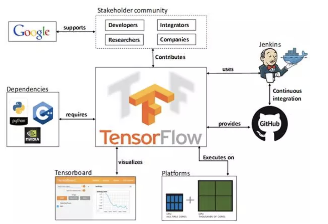
• TF Hosted in github platform , Yes google groups and contributors Jointly maintain .
• TF Provides rich in-depth learning related API, Support Python and C/C++ Interface .
• TF Provides visual analysis tools Tensorboard, It is convenient to analyze and adjust the model .
• TF Support Linux platform ,Windows platform ,Mac platform , Even mobile devices and other platforms .

TensorFlow 2.0 Will focus on simplicity and ease of use , The workflow is as follows ：

1、 Use tf.data Load data . Use tf.data Instantiate and read training data and test data

2、 Model establishment and debugging ： Use dynamic graph mode Eager Execution And the famous neural network API frame Keras, Combined with visualization tools TensorBoard, Simple and easy 、 Quickly build and debug models ;

3、 Model training ： Support CPU / single GPU / Single machine multi card GPU / Multi machine cluster / TPU Training models , Make full use of massive data and computing resources for efficient training ;

4、 Pre training model call ： adopt TensorFlow Hub, It can easily call the existing mature model after pre training .

5、 Model deployment ： adopt TensorFlow Serving、TensorFlow Lite、TensorFlow.js And so on , Can be TensorFlow Deploy the model to the server 、 Mobile 、 Embedded end and other use scenarios ;

1.2 TensorFlow Installation

install TensorFlow stay 64 Test these system support on bit systems TensorFlow：

• Ubuntu 16.04 Or later
• Windows 7 Or later
• macOS 10.12.6 (Sierra) Or later （ I won't support it GPU）

Enter the virtual environment and install . Recommended anoconda Installation

1、 Not GPU Version installed

pip install tensorflow==2.3.0 -i https://pypi.tuna.tsinghua.edu.cn/simple

Even in conda Environment , It is better to use pip Command to install
You can also use conda install tensorflow To install TensorFlow, however conda Source versions tend to update slowly , It is difficult to get the latest at the first time TensorFlow edition ;

from TensorFlow 2.1 Start ,pip package tensorflow That is to say, it includes GPU Support , There's no need to go through a specific pip package tensorflow-gpu install GPU edition . If the pip Packet size sensitivity , You can use tensorflow-cpu Package installation only supports CPU Of TensorFlow edition .

2、GPU Version installation configuration

Recommended reference （Windows Environmental Science ）：https://blog.csdn.net/qq_43108090/article/details/123923212

Two things are mainly installed cuda and cudnn, Pay attention to your own graphics card version , Some old graphics cards do not support the new version TensorFlow Of .

1.3 Tensors and their operations

1.3.1 tensor Tensor

A tensor is a multidimensional array . And NumPy ndarray Objects are similar ,tf.Tensor Object types and shapes also have . As shown in the figure below ：

Besides ,tf.Tensors You can keep it in GPU in . TensorFlow It provides a rich operation Library （tf.add,tf.matmul,tf.linalg.inv etc. ）, They use and generate tf.Tensor. Import the corresponding toolkit before tensor operation ：

import tensorflow as tf
import numpy as np

1. The basic method

First let's create the basic tensor ：

#  establish int32 Type of 0 D tensor , That's scalar 
rank_0_tensor = tf.constant(4)
print(rank_0_tensor)
#  establish float32 Type of 1 D tensor 
rank_1_tensor = tf.constant([2.0, 3.0, 4.0])
print(rank_1_tensor)
#  establish float16 Two dimensional tensor of type 
rank_2_tensor = tf.constant([[1, 2],
                             [3, 4],
                             [5, 6]], dtype=tf.float16)
print(rank_2_tensor)

The output is ：

tf.Tensor(4, shape=(), dtype=int32)
tf.Tensor([2. 3. 4.], shape=(3,), dtype=float32)
tf.Tensor(
[[1. 2.]
 [3. 4.]
 [5. 6.]], shape=(3, 2), dtype=float16)

We can also create higher dimensional tensors ：

#  establish float32 Tensor of type 
rank_3_tensor = tf.constant([
  [[0, 1, 2, 3, 4],
   [5, 6, 7, 8, 9]],
  [[10, 11, 12, 13, 14],
   [15, 16, 17, 18, 19]],
  [[20, 21, 22, 23, 24],
   [25, 26, 27, 28, 29]],])

print(rank_3_tensor)

We have more ways to show this output ：

2. convert to numpy

We can convert the tensor to numpy Medium ndarray In the form of , There are two conversion methods , In tensor rank_2_tensor For example ：

• np.array

np.array(rank_2_tensor)

• Tensor.numpy()

rank_2_tensor.numpy()

3. Common functions

We can do some basic mathematical operations on tensors , Including addition 、 Element multiplication and matrix multiplication ：

#  Define tensor a and b
a = tf.constant([[1, 2],
                 [3, 4]])
b = tf.constant([[1, 1],
                 [1, 1]]) 

print(tf.add(a, b), "\n") #  Calculate the sum of tensors 
print(tf.multiply(a, b), "\n") #  Calculate the element multiplication of the tensor 
print(tf.matmul(a, b), "\n") #  Calculate multiplication 

The output is ：

tf.Tensor(
[[2 3]
 [4 5]], shape=(2, 2), dtype=int32) 

tf.Tensor(
[[1 2]
 [3 4]], shape=(2, 2), dtype=int32) 

tf.Tensor(
[[3 3]
 [7 7]], shape=(2, 2), dtype=int32) 

In addition, tensors can also be used in various aggregation operations ：

tf.reduce_sum()  #  Sum up 
tf.reduce_mean() #  Average 
tf.reduce_max()  #  Maximum 
tf.reduce_min()  #  minimum value 
tf.argmax() #  Index of maximum value 
tf.argmin() #  Index of minimum value 

for example ：

c = tf.constant([[4.0, 5.0], [10.0, 1.0]])
#  Maximum 
print(tf.reduce_max(c))
#  Maximum index 
print(tf.argmax(c))
#  Calculate the mean 
print(tf.reduce_mean(c))

Output is ：

tf.Tensor(10.0, shape=(), dtype=float32)
tf.Tensor([1 0], shape=(2,), dtype=int64)
tf.Tensor(5.0, shape=(), dtype=float32)

4. Variable

A variable is a special tensor , Shape is immutable , The parameters can be changed . The method of definition is ：

my_variable = tf.Variable([[1.0, 2.0], [3.0, 4.0]])

We can also get its shape , Type and convert to ndarray:

print("Shape: ",my_variable.shape)
print("DType: ",my_variable.dtype)
print("As NumPy: ", my_variable.numpy)

Output is ：

Shape:  (2, 2)
DType:  <dtype: 'float32'>
As NumPy:  <bound method BaseResourceVariable.numpy of <tf.Variable 'Variable:0' shape=(2, 2) dtype=float32, numpy=
array([[1., 2.],
       [3., 4.]], dtype=float32)>>

1.4 tf.keras Introduce

tf.keras yes TensorFlow 2.0 Higher order of API Interface , by TensorFlow The code provides new styles and design patterns , Greatly improved TF The simplicity and reusability of the code , It is also officially recommended tf.keras For model design and development .

1.4.1 Common modules

tf.keras The common modules in are shown in the following table ：

1.4.2 Common methods

The main process of deep learning implementation ：1. Data acquisition ,2, Data processing ,3. Model creation and training ,4 Model testing and evaluation ,5. Model to predict

1. Import tf.keras

Use tf.keras, First you need to import... At the beginning of the code tf.keras

import tensorflow as tf
from tensorflow import keras

2. data input

For small data sets , You can use it directly numpy Format data for training 、 Evaluation model , For large data sets or for cross device training tf.data.datasets To enter data .

3. model building

• Simple model use Sequential Build
• Complex models are built using functional programming
• Customize layers

4. Training and evaluation

• Configure the training process ：

#  Configuration optimization method , Loss function and evaluation index 
model.compile(optimizer=tf.train.AdamOptimizer(0.001),
              loss='categorical_crossentropy',
              metrics=['accuracy'])

• model training

#  Indicates the training data set , Training epoch, Batch size and validation set data 
model.fit/fit_generator(dataset, epochs=10, 
                        batch_size=3,
          validation_data=val_dataset,
          )

• Model to evaluate

#  Indicate the evaluation dataset and batch size 
model.evaluate(x, y, batch_size=32)

• Model to predict

#  Predict new samples 
model.predict(x, batch_size=32)

5. Callback function （callbacks）

The callback function is used in the process of model training , To control model training behavior , You can customize the callback function , You can also use tf.keras.callbacks Built in callback ：

ModelCheckpoint： Keep regularly checkpoints. LearningRateScheduler： Dynamically change the learning rate . EarlyStopping： When the performance on the validation set is no longer improved , Stop training . TensorBoard： Use TensorBoard Monitor the status of the model .

6. Model saving and recovery

• Save only parameters

#  Save only the weight of the model 
model.save_weights('./my_model')
#  Load the weight of the model 
model.load_weights('my_model')

• Save the entire model

#  Save the model structure and weight in h5 In file 
model.save('my_model.h5')
#  Load model ： Including the architecture and corresponding weights 
model = keras.models.load_model('my_model.h5')

---

summary

• understand Tensorflow2.0 The purpose and process of the framework
  1. Use tf.data Load data
  2、 Model establishment and debugging
  3、 Model training
  4、 Pre training model call
  5、 Model deployment

• know tf2.0 And its operation
  Tensors are multidimensional arrays .
  1、 Create method ：tf.constant()
  2、 Convert to numpy: np.array() or tensor.asnumpy()
  3、 Common functions ： Add , Multiplication , And various aggregation operations
  4、 Variable ：tf.Variable()

• know tf.keras Related modules and common methods in
  Common modules ：models,losses,application etc.
  Common methods ：

  1、 Import tf.keras
  
  2、 data input 
  
  3、 model building 
  
  4、 Training and evaluation 
  
  5、 Callback function 
  
  6、 The preservation and recovery of the model 
  

Two 、 Quick start model

Today we pass the case of iris classification , Let's introduce tf.keras The basic use process of .tf.keras Use tensorflow High level interface in , We call it to complete ：

1. Import and parse datasets
2. Build the model
3. The model is trained with sample data
4. Evaluate the effectiveness of the model .

Because of and scikit -learn The similarity of , Next we will pass Keras And scikit -learn Compare , Introduce tf.Keras How to use it .

1. Import of related libraries

Use it here sklearn and tf.keras Complete iris classification , Import related Toolkits ：

#  mapping 
import seaborn as sns
#  Numerical calculation 
import numpy as np
# sklearn Related tools in 
#  Divide the training set and the test set 
from sklearn.model_selection import train_test_split
#  Logical regression 
from sklearn.linear_model import LogisticRegressionCV
# tf.keras Related tools used in 
#  For model building 
from tensorflow.keras.models import Sequential
#  Layers and activation methods for building models 
from tensorflow.keras.layers import Dense, Activation
#  Auxiliary tools for data processing 
from tensorflow.keras import utils

2. Data display and division

utilize seborn Import related data ,iris The data to dataFrame The way in seaborn For storage , We read it and show it ：

#  Reading data 
iris = sns.load_dataset("iris")
#  Show the top five elements of the data 
iris.head()

in addition , utilize seaborn in pairplot Function to explore the relationship between data features ：

#  Visualize the relationship between data 
sns.pairplot(iris, hue='species')

Divide the data into training set and test set ： from iris dataframe Extract raw data from , Save the petal and sepal data in an array X in , The tag is stored in the corresponding array y in ：

#  Data of petals and calyx 
X = iris.values[:, :4]
#  Label value 
y = iris.values[:, 4]

utilize train_test_split Complete data set partitioning ：

#  Divide the data set into training set and test set 
train_X, test_X, train_y, test_y = train_test_split(X, y, train_size=0.5, test_size=0.5, random_state=0)

Next , We can use sklearn and tf.keras To complete the forecast

3. sklearn Realization

Using the classifier of logistic regression , The method of cross validation is used to select the optimal hyperparameter , Instantiation LogisticRegressionCV classifier , And use fit Methods training ：

#  Instantiate classifiers 
lr = LogisticRegressionCV()
#  Training 
lr.fit(train_X, train_y)

Use the trained classifier to predict , And calculate the accuracy ：

#  Calculate the accuracy and print 
print("Accuracy = {:.2f}".format(lr.score(test_X, test_y)))

The accuracy of logistic regression is ：

Accuracy = 0.93

4. tf.keras Realization

stay sklearn In, we just instantiate the classifier and use fit Methods training , Finally, measure its performance , That's in tf.keras In and in sklearn Very similar , The difference is ：

• When building a classifier, you need to build a model
• Data collection ,sklearn Can receive string type labels , Such as ：“setosa”, But in tf.keras You need to heat code the tag value in , As shown below ：

There are many ways to implement hot coding , such as pandas Medium get_dummies(), Here we use tf.keras The method in ：

#  Heat code 
def one_hot_encode_object_array(arr):
    #  To retrieve all categories 
    uniques, ids = np.unique(arr, return_inverse=True)
    #  Return the result of hot coding 
    return utils.to_categorical(ids, len(uniques))

4.1 Data processing

Next, heat code the tag values ：

#  Training set heat coding 
train_y_ohe = one_hot_encode_object_array(train_y)
#  Test collector code 
test_y_ohe = one_hot_encode_object_array(test_y)

4.2 Model structures,

stay sklearn in , Models are readily available .tf.Keras Is a neural network library , We need to build neural networks based on data and tag values . Neural network can find the complex relationship between features and labels . A neural network is a highly structured graph , It contains one or more hidden layers . Each hidden layer contains one or more neurons . There are many kinds of neural networks , The program uses a dense neural network , Also known as fully connected neural networks ： Neurons in one layer will take input connections from each neuron in the upper layer . for example , chart 2 Shows a dense neural network , It includes 1 Input layers 、2 A hidden layer and 1 Output layers , As shown in the figure below ：

Upper figure When the model in is trained and fed unlabeled samples , It produces 3 A prediction ： The possibility of iris belonging to the designated species . For this example , The sum of the output predictions is 1.0. The forecast results are decomposed as follows ： Iris is 0.02, Iris discolor is 0.95, Virginia iris is 0.03. This means that the probability of the model predicting that an unlabeled iris sample is a color changing iris is 95％.

TensorFlow tf.keras API Is the preferred way to create models and layers . Through the API, You can easily build models and experiment with them , And the complex work of connecting all the parts is done by Keras Handle .

tf.keras.Sequential Models are linear stacks of layers . The constructor of the model takes a series of layer instances ; In this example , It's using 2 A dense layer （ Each contains 10 Nodes ） as well as 1 Output layers （ contain 3 Nodes representing label prediction ）. The first layer is input_shape Parameters correspond to the number of features in the dataset ：

#  utilize sequential How to build models 
model = Sequential([
  #  Hidden layer 1, The activation function is relu, The input size has input_shape Appoint 
  Dense(10, activation="relu", input_shape=(4,)),  
  #  Hidden layer 2, The activation function is relu
  Dense(10, activation="relu"),
  #  Output layer 
  Dense(3,activation="softmax")
])

adopt model.summary You can view the schema of the model ：

Model: "sequential"
_________________________________________________________________
Layer (type)                 Output Shape              Param #   
=================================================================
dense (Dense)                (None, 10)                50        
_________________________________________________________________
dense_1 (Dense)              (None, 10)                110       
_________________________________________________________________
dense_2 (Dense)              (None, 3)                 33        
=================================================================
Total params: 193
Trainable params: 193
Non-trainable params: 0
_________________________________________________________________             

The activation function determines the output shape of each node in the layer . These nonlinear relationships are important , Without them , The model will be equivalent to a single layer . There are many activation functions , But hidden layers usually use ReLU.

The ideal number of hidden layers and neurons depends on the problem and the data set . Like many aspects of machine learning , Choosing the best shape of neural network needs a certain level of knowledge and experimental basis . Generally speaking , Increasing the number of hidden layers and neurons usually leads to more powerful models , And it takes more data to train effectively .

4.3 Model training and prediction

In the training and evaluation phase , We all need to calculate the loss of the model . This can be used to measure how far the predicted results of the model deviate from the expected labels , in other words , How bad is the model . We want to reduce or optimize this value as much as possible , So we set the optimization strategy and loss function , And the calculation method of model accuracy ：

#  Set relevant parameters of the model ： Optimizer , Loss function and evaluation index 
model.compile(optimizer='adam', loss='categorical_crossentropy', metrics=["accuracy"])

Next, with the sklearn In the same way , Respectively called fit and predict Method to predict .

#  model training ：epochs, The number of times the training samples are sent into the network ,batch_size: The number of samples sent into the network each time 
model.fit(train_X, train_y_ohe, epochs=10, batch_size=1, verbose=1);

The above code completes ：

1. Iterate over each epoch. One pass through a data set is a epoch.
2. In a epoch in , Ergodic training Dataset Each sample in , And obtain the characteristics of the sample (x) And labels (y).
3. Predict according to the characteristics of the sample , And compare the predictions with the labels . Measuring the inaccuracy of predictions , The loss and gradient of the model are calculated using the obtained values .
4. Use optimizer Update the variables of the model .
5. For each epoch Repeat the above steps , Until the model training is completed .

• About epoch：https://blog.csdn.net/u013041398/article/details/72841854
• n individual epoch It means that each sample should be put in n Time

The training process is shown below ：

Epoch 1/10
75/75 [==============================] - 0s 616us/step - loss: 0.0585 - accuracy: 0.9733
Epoch 2/10
75/75 [==============================] - 0s 535us/step - loss: 0.0541 - accuracy: 0.9867
Epoch 3/10
75/75 [==============================] - 0s 545us/step - loss: 0.0650 - accuracy: 0.9733
Epoch 4/10
75/75 [==============================] - 0s 542us/step - loss: 0.0865 - accuracy: 0.9733
Epoch 5/10
75/75 [==============================] - 0s 510us/step - loss: 0.0607 - accuracy: 0.9733
Epoch 6/10
75/75 [==============================] - 0s 659us/step - loss: 0.0735 - accuracy: 0.9733
Epoch 7/10
75/75 [==============================] - 0s 497us/step - loss: 0.0691 - accuracy: 0.9600
Epoch 8/10
75/75 [==============================] - 0s 497us/step - loss: 0.0724 - accuracy: 0.9733
Epoch 9/10
75/75 [==============================] - 0s 493us/step - loss: 0.0645 - accuracy: 0.9600
Epoch 10/10
75/75 [==============================] - 0s 482us/step - loss: 0.0660 - accuracy: 0.9867

And sklearn Different from , When evaluating a trained model , And sklearn.score The method corresponds to tf.keras.evaluate() Method , Returns the loss function and in compile Indicators required when modeling :

#  Calculate the loss and accuracy of the model 
loss, accuracy = model.evaluate(test_X, test_y_ohe, verbose=1)
print("Accuracy = {:.2f}".format(accuracy))

The accuracy of the classifier is ：

3/3 [==============================] - 0s 591us/step - loss: 0.1031 - accuracy: 0.9733
Accuracy = 0.97

Here we are tf.kears Have a basic understanding of the use of , In the next course, we will explain the neural network and the commonly used in computer vision CNN Use .