当前位置:网站首页>TASK03|概率论
TASK03|概率论
2022-06-25 10:20:00 【speoki】
目录
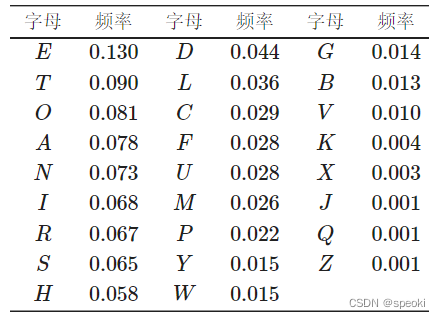
(1)英文写作中的频率表
随机现象与概率
概率论主要研究能大量重复的随机现象‘
(1)随机试验:可重复的随机现象又称为随机试验
(2)样本点:一切可能发生的基本结果
(3)样本空间:随机现象所有基本结果(样本点)的全体称为这个随机现象的样本空间
(4)随机事件:随机现象的某些基本结果组成的集合称为随机事件
(5)事件间的关系:
- 包含
- 相等
- 互不相容
- 必然与不可能事件
(6)事件的运算: - 对立
- 并
- 交
- 差
(7)概率的公理化定义: - 非负性公理
- 正则性公理
- 可加性公理
(8)事件的独立性
模拟频率近似概率
import numpy as np
import pandas as pd
import matplotlib.pyplot as plt
%matplotlib inline
#提供了和 MATLAB 类似的绘图 API
#调用matplotlib.pyplot的绘图函数plot()进行绘图的时候,或者生成一个figure画布的时候,可以直接在你的python console里面生成图像。
plt.style.use("ggplot")
# 画布风格 使用plt.style.available可以找适合图形的风格
import warnings
warnings.filterwarnings("ignore")
#忽略代码中的红色警告
plt.rcParams['font.sans-serif']=['SimHei','Songti SC','STFangsong']
#定义图形默认属性 设置字体
plt.rcParams['axes.unicode_minus']=False
#用来正常显示负号
import seaborn as sns
import random
def Simulate_coin(test_num):
random_seed(100)#定义随机数种子
coin_list=[1 if random.random()>=0.5]else 0 for i range(test_num)]#模拟试验结果
#大于等于0.5的算1 否则算0
coin_frequence = np.cumsum(coin_list)/(np.arrange(len(coin_list))+1)
#计算正面为1的概率
plt.figure(figsize=(10,6))
#绘图,指定画布的大小
plt.plot(np.arrange(len(coin_list))+1,coin_frequence,c='blue',alpha=0.7)
#横坐标测验的次数,纵坐标频度
plt.xlabel("test_index")
plt.ylabel("frequence")
plt.title(str(test_num)+" times")
plt.show()
Simulate_coin(test_num = 600)
Simulate_coin(test_num = 1000)
Simulate_coin(test_num = 6000)
Simulate_coin(test_num = 10000)
条件概率,乘法公式,全概率公式与贝叶斯公式
(1)条件概率
P ( A ∣ B ) = P ( A B ) P ( B ) P(A \mid B)=\frac{P(A B)}{P(B)} P(A∣B)=P(B)P(AB)
(2)乘法公式
- 若 P ( B ) > 0 P(B)>0 P(B)>0, 则 P ( A B ) = P ( B ) P ( A ∣ B ) P(A B)=P(B) P(A \mid B) P(AB)=P(B)P(A∣B)
- 若 P ( A 1 A 2 ⋯ A n − 1 ) > 0 P\left(A_{1} A_{2} \cdots A_{n-1}\right)>0 P(A1A2⋯An−1)>0, 则 P ( A 1 A 2 ⋯ A n ) = P ( A 1 ) P ( A 2 ∣ A 1 ) P ( A 3 ∣ A 1 A 2 ) ⋯ P ( A n ∣ A 1 A 2 ⋯ A n − 1 ) P\left(A_{1} A_{2} \cdots A_{n}\right)=P\left(A_{1}\right) P\left(A_{2} \mid A_{1}\right) P\left(A_{3} \mid A_{1} A_{2}\right) \cdots P\left(A_{n} \mid A_{1} A_{2} \cdots A_{n-1}\right) P(A1A2⋯An)=P(A1)P(A2∣A1)P(A3∣A1A2)⋯P(An∣A1A2⋯An−1)
exp:
P ( A ˉ 1 A ˉ 2 A 3 ) = P ( A ˉ 1 ) P\left(\bar{A}_{1} \bar{A}_{2} A_{3}\right)=P\left(\bar{A}_{1}\right) P(Aˉ1Aˉ2A3)=P(Aˉ1)
P ( A ˉ 2 ∣ A ˉ 1 ) P ( A 3 ∣ A ˉ 1 A ˉ 2 ) = 90 100 ⋅ 89 99 ⋅ 10 98 = 0.0826. P\left(\bar{A}_{2} \mid \bar{A}_{1}\right) P\left(A_{3} \mid \bar{A}_{1} \bar{A}_{2}\right)=\frac{90}{100} \cdot \frac{89}{99} \cdot \frac{10}{98}=0.0826 . P(Aˉ2∣Aˉ1)P(A3∣Aˉ1Aˉ2)=10090⋅9989⋅9810=0.0826.
(3)全概率公式
P ( A ) = ∑ i = 1 n P ( A ∣ B i ) P ( B i ) P(A)=\sum_{i=1}^{n} P\left(A \mid B_{i}\right) P\left(B_{i}\right) P(A)=i=1∑nP(A∣Bi)P(Bi)

(4)贝叶斯公式
用简单的 P ( A ∣ B k ) P\left(A \mid B_{k}\right) P(A∣Bk)求解复杂的 P ( B k ∣ A ) P\left(B_{k} \mid A\right) P(Bk∣A)
P ( B k ∣ A ) = P ( A B k ) P ( A ) P\left(B_{k} \mid A\right) = \frac{P(AB_k)}{P(A)} P(Bk∣A)=P(A)P(ABk)
对分子分母分别使用乘法公式和全概率公式展开,即:
P ( B k ∣ A ) = P ( A ∣ B k ) P ( B k ) ∑ i = 1 n P ( A ∣ B i ) P ( B i ) , k = 1 , 2 , ⋯ , n P\left(B_{k} \mid A\right)=\frac{P\left(A \mid B_{k}\right) P\left(B_{k}\right)}{\sum_{i=1}^{n} P\left(A \mid B_{i}\right) P\left(B_{i}\right)}, \quad k=1,2, \cdots, n P(Bk∣A)=∑i=1nP(A∣Bi)P(Bi)P(A∣Bk)P(Bk),k=1,2,⋯,n
三门问题
参赛者会看见三扇关闭了的门,其中一扇的后面有一辆汽车,选中后面有车的那扇门就可以赢得该汽车,而另外两扇门后面则各藏有1只山羊。当参赛者选定了一扇门,但未去开启它的时候,节目主持人会开启剩下两扇门的其中一扇,露出其中1只山羊。主持人其后会问参赛者要不要换另一扇仍然关上的门。问题是:换另一扇门会否增加参赛者赢得汽车的机率?
在主持人不打开门时, 选手抽中车的概率为 1 / 3 1 / 3 1/3
P ( A ) = P ( B ) = P ( C ) = 1 / 3 \begin{aligned} &P(A)=P(B)=P(C)=1 / 3\\ \end{aligned} P(A)=P(B)=P(C)=1/3
假设:
A: 选手选择第二扇门,第一扇门是车,
B: 选手选择第二扇门,第二扇门是车,
C: 选手选择第二扇门,第三扇门是车,
D: 主持人打开第一扇门
根据语义我们可以列出概率公式
P ( D ∣ A ) = 0 P ( D ∣ B ) = 1 / 2 P ( D ∣ C ) = 1 \begin{aligned} P(D|A)=0 P(D|B)=1/2 P(D|C)=1 \end{aligned} P(D∣A)=0P(D∣B)=1/2P(D∣C)=1
根据贝叶斯公式: P ( D ) = P ( A ) P ( D ∣ A ) + P ( B ) P ( D ∣ B ) + P ( C ) P ( D ∣ C ) = 1 / 2 P ( C ∣ D ) = P ( C ) P ( D ∣ C ) / P ( D ) = 2 / 3 P ( B ∣ D ) = P ( B ) P ( D ∣ B ) / P ( D ) = 1 / 3 \begin{aligned} &\text{根据贝叶斯公式:}\\ &P(D)=P(A) P(D \mid A)+P(B) P(D \mid B)+P(C) P(D \mid C)=1 / 2 \\ &P(C \mid D)=P(C) P(D \mid C) / P(D)=2 / 3 \\ &P(B \mid D)=P(B) P(D \mid B) / P(D)=1 / 3 \end{aligned} 根据贝叶斯公式:P(D)=P(A)P(D∣A)+P(B)P(D∣B)+P(C)P(D∣C)=1/2P(C∣D)=P(C)P(D∣C)/P(D)=2/3P(B∣D)=P(B)P(D∣B)/P(D)=1/3
import random
class MontyHall:
  def __init__(self,n): #构造函数
	self.n=n#试验的次数
	self.change=0#记录换才能拿到车的次数
	sellf.No_change=0#不换
  def start(self):
	for i in range(self,n):
		door_list=[1,2,3]#三扇门
		challenger_door = random.choice(door_list)
		##随机选择了其中一扇
		car_door=  random.choice(door_list)
		#车的门
		##没有被挑战者选中的剩下的门
		door_list.remove(challenger_door)

		if challenger_door==car_door:
			host_door = random.choice(door_list)
			door.remove(host_door)
		#不换才能拿车
			self.No_change+=1
		else:
			self.change+=1
		#换了才能拿车
		  print("换且能拿到车的概率:%.2f " % (self.change/self.n * 100) + "%")
        print("不换也能拿到车的概率:%.2f"% (self.No_change/self.n * 100) + "%")

if __name__ == "__main__":
    mh = MontyHall(1000000)
    mh.start()
一维随机变量
随机变量分为离散的和连续的
计算一个由随机变量表示的随机事件的概率的思路有两种:直接计算法(利用分布函数计算) 和 间接计算法(利用密度函数计算)
F ( x ) = P ( X ⩽ x ) F(x)=P(X \leqslant x) F(x)=P(X⩽x)
0 ⩽ F ( x ) ⩽ 1 0 \leqslant F(x) \leqslant 1 0⩽F(x)⩽1
- F ( − ∞ ) = lim x → − ∞ F ( x ) = 0 F(-\infty)=\lim _{x \rightarrow-\infty} F(x)=0 F(−∞)=limx→−∞F(x)=0 ,这是因为事件“ X ⩽ − ∞ X \leqslant-\infty X⩽−∞ "是不可能事件。
- F ( + ∞ ) = lim x → + ∞ F ( x ) = 1 F(+\infty)=\lim _{x \rightarrow+\infty} F(x)=1 F(+∞)=limx→+∞F(x)=1, 这是因为事件“ X ⩽ + ∞ X \leqslant+\infty X⩽+∞ "是必然事件。
P ( a < X ⩽ b ) = F ( b ) − F ( a ) P ( X = a ) = F ( a ) − F ( a − 0 ) P ( X ⩾ b ) = 1 − F ( b − 0 ) P ( X > b ) = 1 − F ( b ) P ( X < b ) = F ( b − 0 ) P ( a < X < b ) = F ( b − 0 ) − F ( a ) P ( a ⩽ X ⩽ b ) = F ( b ) − F ( a − 0 ) P ( a ⩽ X < b ) = F ( b − 0 ) − F ( a − 0 ) \begin{aligned} &P(a<X \leqslant b)=F(b)-F(a) \\ &P(X=a)=F(a)-F(a-0) \\ &P(X \geqslant b)=1-F(b-0) \\ &P(X>b)=1-F(b)\\ &P(X<b)=F(b-0) \\ &P(a<X<b)=F(b-0)-F(a) \\ &P(a \leqslant X \leqslant b)=F(b)-F(a-0) \\ &P(a \leqslant X<b)=F(b-0)-F(a-0) \end{aligned} P(a<X⩽b)=F(b)−F(a)P(X=a)=F(a)−F(a−0)P(X⩾b)=1−F(b−0)P(X>b)=1−F(b)P(X<b)=F(b−0)P(a<X<b)=F(b−0)−F(a)P(a⩽X⩽b)=F(b)−F(a−0)P(a⩽X<b)=F(b−0)−F(a−0)
a a a 与 b b b 处连续时, 有
F ( a − 0 ) = F ( a ) , F ( b − 0 ) = F ( b ) F(a-0)=F(a), \quad F(b-0)=F(b) F(a−0)=F(a),F(b−0)=F(b)
利用密度函数计算某个区域内的概率
P ( a ⩽ X ⩽ b ) = ∫ a b p ( x ) d x P(a \leqslant X \leqslant b)=\int_{a}^{b} p(x) d x P(a⩽X⩽b)=∫abp(x)dx
离散型 :
分布列
X x 1 x 2 ⋯ x n ⋯ P p ( x 1 ) p ( x 2 ) ⋯ p ( x n ) ⋯ \begin{array}{c|ccccc} X & x_{1} & x_{2} & \cdots & x_{n} & \cdots \\ \hline P & p\left(x_{1}\right) & p\left(x_{2}\right) & \cdots & p\left(x_{n}\right) & \cdots \end{array} XPx1p(x1)x2p(x2)⋯⋯xnp(xn)⋯⋯
连续型:
exp:
柯西分布的密度函数,对分布函数求导
## 已知柯西分布的密度函数求分布函数
from sympy import *
x = symbols('x')
p_x = 1/pi*(1/(1+x**2))
integrate(p_x,(x,-∞,x))
#积分 从负无穷到x

from sympy import *
x = symbols('x')
f_x = 1/pi*(atan(x)+pi/2)
diff(f_x,x,1)
#求导
均匀分布:
密度函数为
U ( a , b ) U(a, b) U(a,b)
p ( x ) = { 1 b − a , a ⩽ x ⩽ b 0 , 其它 p(x)= \begin{cases}\frac{1}{b-a}, & a \leqslant x \leqslant b \\ 0, & \text { 其它 }\end{cases} p(x)={ b−a1,0,a⩽x⩽b 其它
分布函数为:
F ( x ) = { 0 , x < a x − a b − a , a ⩽ x < b 1 , x ⩾ b F(x)= \begin{cases}0, & x<a \\ \frac{x-a}{b-a}, & a \leqslant x<b \\ 1, & x \geqslant b\end{cases} F(x)=⎩⎪⎨⎪⎧0,b−ax−a,1,x<aa⩽x<bx⩾b
exp:
a = float(0)
b = float(1)
#numpy.linspace()函数用于在线性空间中以均匀步长生成数字序列
x = np.linspace(a,b)
y = np.full(shape=len(x),fill_value=1/(b-a))
#np.full构造一个数组
plt.plot(x,y,"b",linewidth=2)
plt.ylim(0,1,2)
plt.xlim(-1,2)
plt.xlabel('X')
plt.ylabel('p(x)')
plt.title('uniform distribution')
plt.show()

指数分布
p ( x ) = { λ e − λ x , x ⩾ 0 0 , x < 0 p(x)=\left\{\begin{aligned} \lambda e^{-\lambda x}, & x \geqslant 0 \\ 0, & x<0 \end{aligned}\right. p(x)={ λe−λx,0,x⩾0x<0
F ( x ) = { 1 − e − λ x , x ⩾ 0 0 , x < 0 F(x)= \begin{cases}1-\mathrm{e}^{-\lambda x}, & x \geqslant 0 \\ 0, & x<0\end{cases} F(x)={ 1−e−λx,0,x⩾0x<0
lam = float(1.5)
x = np.linspace(0,15,100)
y = lam*np.e**(-lam*x)

plt.plot(x,y,"b",linewidth=2)
plt.xlim(-5,10)
plt.xlabel('X')
plt.ylabel('p(x)')
plt.title('指数分布')
plt.show()

高斯分布

from sympy import *
from sympy.abc import mu,sigma
x = symbols('X')
p_x = 1/(sqer(2*pi)*sigma)*E**(-(x-mu)**2/(2*sigma**2))
integrate(p_x,(x,-∞,x))

import math
mu = float(0)
mul = float(2)
sigma1 = float(1)
sigma2 = float(1.25)*float(1.25)
sigma3 = float(0.25)
x = np.linspace(-5, 5, 1000)
y1 = np.exp(-(x - mu)**2 / (2 * sigma1**2)) / (math.sqrt(2 * math.pi) * sigma1)
y2 = np.exp(-(x - mu)**2 / (2 * sigma2**2)) / (math.sqrt(2 * math.pi) * sigma2)
y3 = np.exp(-(x - mu)**2 / (2 * sigma3**2)) / (math.sqrt(2 * math.pi) * sigma3)
y4 = np.exp(-(x - mu1)**2 / (2 * sigma1**2)) / (math.sqrt(2 * math.pi) * sigma1)
plt.plot(x,y1,"b",linewidth=2,label=r'$\mu=0,\sigma=1$')
plt.plot(x,y2,"orange",linewidth=2,label=r'$\mu=0,\sigma=1.25$')
plt.plot(x,y3,"yellow",linewidth=2,label=r'$\mu=0,\sigma=0.5$')
plt.plot(x,y4,"b",linewidth=2,label=r'$\mu=2,\sigma=1$',ls='--')
plt.axvline(x=mu,ls='--')
plt.text(x=0.05,y=0.5,s=r'$\mu=0$')
plt.axvline(x=mu1,ls='--')
plt.text(x=2.05,y=0.5,s=r'$\mu=2$')
plt.xlim(-5,5)
plt.xlabel('X')
plt.ylabel('p (x)')
plt.title('normal distribution')
plt.legend()
plt.show()
改变mu


改变σ

指数分布计算
from scipy.stats import expon #指数分布
x = np.linspace(0.01,10,1000)
plt.plot(x,expon.pdf(x),'r-',lw=5,alpha=0.6,label='expon pdf')
 # pdf表示求密度函数值
 # cdf表示求分布函数值
plt.xlabel("X")
plt.ylabel("p (x)")
plt.legend()
#plt.legend创建图例
plt.show()


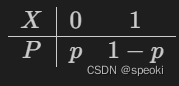
(1)0-1分布
(2)二项分布

(3)泊松分布
泊松分布计算
# 对比不同的lambda对泊松分布的影响
import math
# 构造泊松分布列的计算函数
def poisson(lmd,x):
    return pow(lmd,x)/math.factorial(x)*math.exp(-lmd)
x = [i+1 for i in range(10)]
#定义泊松分布列
lmd1 = 0.8
lmd2 = 2.0
lmd3 = 4.0
lmd4 = 6.0

p_lmd1 = [poisson(lmd1,i) for i in x]
p_lmd2 = [poisson(lmd2,i) for i in x]
p_lmd3 = [poisson(lmd3,i) for i in x]
p_lmd4 = [poisson(lmd4,i) for i in x]

plt.scatter(np.array(x), p_lmd1, c='b',alpha=0.7)
plt.axvline(x=lmd1,ls='--')
plt.text(x=lmd1+0.1,y=0.1,s=r"$\lambda=0.8$")
plt.ylim(-0.1,1)
plt.xlabel("X")
plt.ylabel("p (x)")
plt.title(r"$\lambda = 0.8$")
plt.show()

plt.scatter(np.array(x), p_lmd2, c='b',alpha=0.7)
plt.axvline(x=lmd2,ls='--')
plt.text(x=lmd2+0.1,y=0.1,s=r"$\lambda=2.0$")
plt.ylim(-0.1,1)
plt.xlabel("X")
plt.ylabel("p (x)")
plt.title(r"$\lambda = 2.0$")
plt.show()

plt.scatter(np.array(x), p_lmd3, c='b',alpha=0.7)

plt.axvline(x=lmd3,ls='--')
plt.text(x=lmd3+0.1,y=0.1,s=r"$\lambda=4.0$")
plt.ylim(-0.1,1)
plt.xlabel("X")
plt.ylabel("p (x)")
plt.title(r"$\lambda = 4.0$")
plt.show()

plt.scatter(np.array(x), p_lmd4, c='b',alpha=0.7)
plt.axvline(x=lmd4,ls='--')
plt.text(x=lmd4+0.1,y=0.1,s=r"$\lambda=6.0$")
plt.ylim(-0.1,1)
plt.xlabel("X")
plt.ylabel("p (x)")
plt.title(r"$\lambda = 6.0$")
plt.show()
plt.scatter散点图
axvline函数作用是绘制一条跨越整个子图的垂直线
ylim设置或查询 y 坐标轴范围
from scipy.stats import binom
#scipy.stats包中的binom类对象是表示二项分布的。
n = 10
p = 0.5
x = np.arange(1,n+1,1)
pList = binom.pmf(x,n,p)
#stats.binom.pmf(X,n,p) 用于求概率密度
plt.plot(x,pList,marker='o',alpha = 0.7,linestyle = 'None')

plt.vlines(x, 0, pList)
#绘制数据集
plt.xlabel('随机变量:抛硬币10次')
plt.ylabel('概率')
plt.title('二项分布:n=%d,p=%0.2f' % (n,p))
plt.show()
一维随机变量的数字特征:期望、方差、分位数与中位数
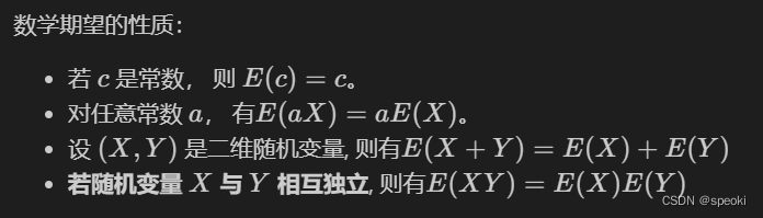
(1)数学期望
分布的位置特征数
离散随机变量:
连续随机变量:
如果积分有限:

exp:

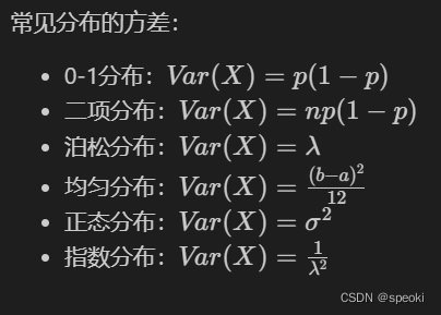
(2)标准差与方差
反应随机变量的波动大小
方差
离散型:
连续型:

标准差
scipy计算常见分布的均值与方差
# 使用scipy计算常见分布的均值与方差:(如果忘记公式的话直接查,不需要查书了)
from scipy.stats import bernoulli   # 0-1分布
from scipy.stats import binom   # 二项分布
from scipy.stats import poisson  # 泊松分布
from scipy.stats import rv_discrete # 自定义离散随机变量
from scipy.stats import uniform # 均匀分布
from scipy.stats import expon # 指数分布
from scipy.stats import norm # 正态分布
from scipy.stats import rv_continuous  # 自定义连续随机变量

print("0-1分布的数字特征:均值:{};方差:{};标准差:{}".format(bernoulli(p=0.5).mean(),
                                  bernoulli(p=0.5).var(),
                                  bernoulli(p=0.5).std()))
print("二项分布b(100,0.5)的数字特征:均值:{};方差:{};标准差:{}".format(binom(n=100,p=0.5).mean(),
                                  binom(n=100,p=0.5).var(),
                                  binom(n=100,p=0.5).std()))
## 模拟抛骰子的特定分布
xk = np.arange(6)+1
pk = np.array([1.0/6]*6)
print("泊松分布P(0.6)的数字特征:均值:{};方差:{};标准差:{}".format(poisson(0.6).mean(),
                                  poisson(0.6).var(),
                                  poisson(0.6).std()))
print("特定离散随机变量的数字特征:均值:{};方差:{};标准差:{}".format(rv_discrete(name='dice', values=(xk, pk)).mean(),
                                  rv_discrete(name='dice', values=(xk, pk)).var(),
                                  rv_discrete(name='dice', values=(xk, pk)).std()))
print("均匀分布U(1,1+5)的数字特征:均值:{};方差:{};标准差:{}".format(uniform(loc=1,scale=5).mean(),
                                  uniform(loc=1,scale=5).var(),
                                  uniform(loc=1,scale=5).std()))
print("正态分布N(0,0.0001)的数字特征:均值:{};方差:{};标准差:{}".format(norm(loc=0,scale=0.01).mean(),
                                  norm(loc=0,scale=0.01).var(),
                                  norm(loc=0,scale=0.01).std()))

lmd = 5.0  # 指数分布的lambda = 5.0
print("指数分布Exp(5)的数字特征:均值:{};方差:{};标准差:{}".format(expon(scale=1.0/lmd).mean(),
                                  expon(scale=1.0/lmd).var(),
                                  expon(scale=1.0/lmd).std()))

## 自定义标准正态分布
class gaussian_gen(rv_continuous):
    def _pdf(self, x): # tongguo
        return np.exp(-x**2 / 2.) / np.sqrt(2.0 * np.pi)
gaussian = gaussian_gen(name='gaussian')
print("标准正态分布的数字特征:均值:{};方差:{};标准差:{}".format(gaussian().mean(),
                                  gaussian().var(),
                                  gaussian().std()))

## 自定义指数分布
import math
class Exp_gen(rv_continuous):
    def _pdf(self, x,lmd):
        y=0
        if x>0:
            y = lmd * math.e**(-lmd*x)
        return y
Exp = Exp_gen(name='Exp(5.0)')
print("Exp(5.0)分布的数字特征:均值:{};方差:{};标准差:{}".format(Exp(5.0).mean(),
                                  Exp(5.0).var(),
                                  Exp(5.0).std()))

## 通过分布函数自定义分布
class Distance_circle(rv_continuous):                 #自定义分布xdist
    """ 向半径为r的圆内投掷一点,点到圆心距离的随机变量X的分布函数为: if x<0: F(x) = 0; if 0<=x<=r: F(x) = x^2 / r^2 if x>r: F(x)=1 """
    def _cdf(self, x, r):                   #累积分布函数定义随机变量
        f=np.zeros(x.size)                  #函数值初始化为0
        index=np.where((x>=0)&(x<=r))           #0<=x<=r
        f[index]=((x[index])/r[index])**2       #0<=x<=r
        index=np.where(x>r)                     #x>r
        f[index]=1                              #x>r
        return f
dist = Distance_circle(name="distance_circle")
print("dist分布的数字特征:均值:{};方差:{};标准差:{}".format(dist(5.0).mean(),
                                  dist(5.0).var(),
                                  dist(5.0).std()))
(3)分位数与中位数
累计概率等于p所对应的随机变量取值x为p分位数
F ( x p ) = ∫ − ∞ x p p ( x ) d x = p F\left(x_{p}\right)=\int_{-\infty}^{x_{p}} p(x) \mathrm{d} x=p F(xp)=∫−∞xpp(x)dx=p

上下侧相互转换转换公式
x p ′ = x 1 − p , x p = x 1 − p ′ x_{p}^{\prime}=x_{1-p}, \quad x_{p}=x_{1-p}^{\prime} xp′=x1−p,xp=x1−p′
中位数就是P=0.5时的分位数点
F ( x 0.5 ) = ∫ − ∞ x 0.5 p ( x ) d x = 0.5 F\left(x_{0.5}\right)=\int_{-\infty}^{x_{0.5}} p(x) \mathrm{d} x=0.5 F(x0.5)=∫−∞x0.5p(x)dx=0.5
中位数和均值可以综合说明数据的分布
均值会受到极端数据的影响
使用python计算标准正态分布的0.25,0.5(中位数),0.75,0.95分位数点。
from scipy.stats import norm
print("标准正态分布的0.25分位数:",norm(loc=0,scale=1).ppf(0.25))   # 使用ppf计算分位数点
print("标准正态分布的0.5分位数:",norm(loc=0,scale=1).ppf(0.5))
print("标准正态分布的0.75分位数:",norm(loc=0,scale=1).ppf(0.75))
print("标准正态分布的0.95分位数:",norm(loc=0,scale=1).ppf(0.95))
多维随机变量及其联合分布、边际分布、条件分布
(1)n维随机变量
(1.1)n维随机变量的联合分布函数
(1.2)n维随机变量的联合密度函数

(1.3)多维离散随机变量联合分布列

# 绘制二维正态分布的联合概率密度曲面图
from scipy.stats import multivariate_normal
from mpl_toolkits.mplot3d import axes3d
# mpl_toolkits.mplot3d画三维图的工具包
x, y = np.mgrid[-5:5:.01, -5:5:.01]  # 返回多维结构
#mgrid用法:返回多维结构
pos = np.dstack((x, y))
#自 x和 y都是二维的,np.dstack通过插入大小为 1 的第三个维度来扩展它们
rv = multivariate_normal([0.5, -0.2], [[2.0, 0.3], [0.3, 0.5]])
# multivariate_normal从多元正态分布中随机抽取样本 的函数
z = rv.pdf(pos)
# pdf求密度函数值
plt.figure('Surface', facecolor='lightgray',figsize=(12,8))
ax = plt.axes(projection='3d')
ax.set_xlabel('X', fontsize=14)
ax.set_ylabel('Y', fontsize=14)
ax.set_zlabel('P (X,Y)', fontsize=14)
ax.plot_surface(x, y, z, rstride=50, cstride=50, cmap='jet')
plt.show()
# 绘制二维正态分布的联合概率密度等高线图
from scipy.stats import multivariate_normal
x, y = np.mgrid[-1:1:.01, -1:1:.01]
pos = np.dstack((x, y))
rv = multivariate_normal([0.5, -0.2], [[2.0, 0.3], [0.3, 0.5]])
z = rv.pdf(pos)
fig = plt.figure(figsize=(8,6))
ax2 = fig.add_subplot(111)
ax2.set_xlabel('X', fontsize=14)
ax2.set_ylabel('Y', fontsize=14)
ax2.contourf(x, y, z, rstride=50, cstride=50, cmap='jet')
plt.show()
(2.1)边际分布函数:
lim y → ∞ F ( x , y ) = P ( X ⩽ x , Y < ∞ ) = P ( X ⩽ x ) , \lim _{y \rightarrow \infty} F(x, y)=P(X \leqslant x, Y<\infty)=P(X \leqslant x), y→∞limF(x,y)=P(X⩽x,Y<∞)=P(X⩽x),
(2.2)边际密度函数
F X ( x ) = F ( x , ∞ ) = ∫ − ∞ x ( ∫ − ∞ ∞ p ( u , v ) d v ) d u = ∫ − ∞ x p X ( u ) d u F Y ( y ) = F ( ∞ , y ) = ∫ − ∞ y ( ∫ − ∞ ∞ p ( u , v ) d u ) d v = ∫ − ∞ y p Y ( v ) d v \begin{aligned} &F_{X}(x)=F(x, \infty)=\int_{-\infty}^{x}\left(\int_{-\infty}^{\infty} p(u, v) \mathrm{d} v\right) \mathrm{d} u=\int_{-\infty}^{x} p_{X}(u) \mathrm{d} u \\ &F_{Y}(y)=F(\infty, y)=\int_{-\infty}^{y}\left(\int_{-\infty}^{\infty} p(u, v) \mathrm{d} u\right) \mathrm{d} v=\int_{-\infty}^{y} p_{Y}(v) \mathrm{d} v \end{aligned} FX(x)=F(x,∞)=∫−∞x(∫−∞∞p(u,v)dv)du=∫−∞xpX(u)duFY(y)=F(∞,y)=∫−∞y(∫−∞∞p(u,v)du)dv=∫−∞ypY(v)dv
# 求边际密度函数 p_{X}(x)
from sympy import *
x = symbols('x')
y = symbols('y')
p_xy = Piecewise((1,And(x>0,x<1,y<x,y>-x)),(0,True))
integrate(p_xy, (y, -oo, oo))   ## 由于0<x<1时候,那么x>-x,即2x

# 求边际密度函数 p_{Y}(y)
integrate(p_xy, (x, -oo, oo))   ## 由于|y|<x,0<x<1时,因此y肯定在(-1,1)
(2.3)边际分布列
x的边际分布列
∑ j = 1 ∞ P ( X = x i , Y = y j ) = P ( X = x i ) , i = 1 , 2 , ⋯ \sum_{j=1}^{\infty} P\left(X=x_{i}, Y=y_{j}\right)=P\left(X=x_{i}\right), \quad i=1,2, \cdots j=1∑∞P(X=xi,Y=yj)=P(X=xi),i=1,2,⋯
y 的边际分布列。
∑ i = 1 ∞ P ( X = x i , Y = y j ) = P ( Y = y j ) , j = 1 , 2 , ⋯ \sum_{i=1}^{\infty} P\left(X=x_{i}, Y=y_{j}\right)=P\left(Y=y_{j}\right), \quad j=1,2, \cdots i=1∑∞P(X=xi,Y=yj)=P(Y=yj),j=1,2,⋯
(3)条件分布


# 求际密度函数 p_{Y}(y)
from sympy import *
from sympy.abc import lamda,m,p,k
x = symbols('x')
y = symbols('y')
f_p = lamda**m/factorial(m)*E**(-lamda)*factorial(m)/(factorial(k)*factorial(m-k))*p**k*(1-p)**(m-k)
summation(f_p, (m, k, +oo))
(3.1)连续场合的全概率公式与贝叶斯公式

多维随机变量的数字特征:期望向量、协方差与协方差矩阵、相关系数与相关系数矩阵、条件期望
(1)期望向量
n n n 维随机向量为 X = ( X 1 , X 2 , ⋯ , X n ) ′ \boldsymbol{X}=\left(X_{1}, X_{2}, \cdots, X_{n}\right)^{\prime} X=(X1,X2,⋯,Xn)′每个分量的数学期望都存在
数学期望向量(一般为列向量)
E ( X ) = ( E ( X 1 ) , E ( X 2 ) , ⋯ , E ( X n ) ) ′ E(\boldsymbol{X})=\left(E\left(X_{1}\right), E\left(X_{2}\right), \cdots, E\left(X_{n}\right)\right)^{\prime} E(X)=(E(X1),E(X2),⋯,E(Xn))′
(2)协方差与协方差矩阵:
(2.1)协方差:
Cov ( X , Y ) = E [ ( X − E ( X ) ) ( Y − E ( Y ) ) ] \operatorname{Cov}(X, Y)=E[(X-E(X))(Y-E(Y))] Cov(X,Y)=E[(X−E(X))(Y−E(Y))]
Cov ( X , Y ) = E ( X Y ) − E ( X ) E ( Y ) \operatorname{Cov}(X, Y)=E(X Y)-E(X) E(Y) Cov(X,Y)=E(XY)−E(X)E(Y)
当 Cov ( X , Y ) > 0 \operatorname{Cov}(X, Y)>0 Cov(X,Y)>0 时, 称 X X X 与 Y Y Y 正相关
当 Cov ( X , Y ) < 0 \operatorname{Cov}(X, Y)<0 Cov(X,Y)<0 时, 称 X X X 与 Y Y Y 负相关
当 Cov ( X , Y ) = 0 \operatorname{Cov}(X, Y)=0 Cov(X,Y)=0 时,称 X X X 与 Y Y Y 不相关
若随机变量 X X X 与 Y Y Y 相互独立, 则 Cov ( X , Y ) = 0 \operatorname{Cov}(X, Y)=0 Cov(X,Y)=0
Cov ( X , Y ) = Cov ( Y , X ) . \operatorname{Cov}(X, Y)=\operatorname{Cov}(Y, X) . Cov(X,Y)=Cov(Y,X).
Cov ( X , a ) = 0 \operatorname{Cov}(X, a)=0 Cov(X,a)=0
Cov ( a X , b Y ) = a b Cov ( X , Y ) . \operatorname{Cov}(a X, b Y)=a b \operatorname{Cov}(X, Y) . Cov(aX,bY)=abCov(X,Y).
Cov ( X + Y , Z ) = Cov ( X , Z ) + Cov ( Y , Z ) \operatorname{Cov}(X+Y, Z)=\operatorname{Cov}(X, Z)+\operatorname{Cov}(Y, Z) Cov(X+Y,Z)=Cov(X,Z)+Cov(Y,Z)
对任意二维随机变量 ( X , Y ) (X, Y) (X,Y), 有
Var ( X ± Y ) = Var ( X ) + Var ( Y ) ± 2 Cov ( X , Y ) \operatorname{Var}(X \pm Y)=\operatorname{Var}(X)+\operatorname{Var}(Y) \pm 2 \operatorname{Cov}(X, Y) Var(X±Y)=Var(X)+Var(Y)±2Cov(X,Y)
exp:
p ( x , y ) = { 3 x , 0 < y < x < 1 , 0 , 其他. p(x, y)= \begin{cases}3 x, & 0<y<x<1, \\ 0, & \text { 其他. }\end{cases} p(x,y)={ 3x,0,0<y<x<1, 其他.
求 Cov ( X , Y ) \operatorname{Cov}(X, Y) Cov(X,Y)。
# 求协方差
from sympy import *
from sympy.abc import lamda,m,p,k
x = symbols('x')
y = symbols('y')
p_xy = Piecewise((3*x,And(y>0,y<x,x<1)),(0,True))
E_xy = integrate(x*y*p_xy, (x, -oo, oo),(y,-oo,oo))
E_x = integrate(x*p_xy, (x, -oo, oo),(y,-oo,oo))
E_y = integrate(y*p_xy, (x, -oo, oo),(y,-oo,oo))
E_xy - E_x*E_y
边栏推荐
- How to install SSL certificates in Microsoft Exchange 2010
- P2P network core technology: Gossip protocol
- [paper reading | deep reading] line: large scale information network embedding
- [RPC] i/o model - Rector mode of bio, NiO, AIO and NiO
- 【图像融合】基于形态学分析结合稀疏表征实现图像融合附matlab代码
- ShardingSphere-Proxy 5.0 分库分表(一)
- How to develop wechat applet? How to open a wechat store
- 单片机进阶---PCB开发之照葫芦画瓢(二)
- 手机办理广州证券开户靠谱安全吗?
- [200 opencv routines] 210 Are there so many holes in drawing a straight line?
猜你喜欢

Principle of distribution: understanding the gossip protocol

Houdini graphic notes: could not create OpenCL device of type (houdini_ocl_devicetype) problem solving

Network protocol learning -- lldp protocol learning

ShardingSphere-Proxy 5.0 分库分表(一)

【RPC】I/O模型——BIO、NIO、AIO及NIO的Rector模式
Shardingsphere proxy 5.0 sub database and sub table (I)

单片机开发---基于ESP32-CAM的人脸识别应用

How to do the wechat selling applet? How to apply for applets

西门子PLCS7-200使用(一)---开发环境和组态软件入门

Bitmap is converted into drawable and displayed on the screen
随机推荐
WPF prism framework
Shardingsphere proxy 5.0 sub database and sub table (I)
Linked list delete nodes in the linked list
【论文阅读|深度】Role-based network embedding via structural features reconstruction with degree-regularized
DigiCert和GlobalSign单域名OV SSL证书对比评测
Modbus protocol and serialport port read / write
持续交付-Jenkinsfile 语法
Webapi performance optimization
Solutions using protobuf in TS projects
Opencv learning (I) -- environment building
XSS攻击
Shardingsphere proxy 4.1 sub database and sub table
Request&Response有这一篇就够了
How much does a wechat applet cost? Wechat applet development and production costs? Come and have a look
我希望按照我的思路尽可能将canvas基础讲明白
数组结构整理
Houdini图文笔记:Could not create OpenCL device of type (HOUDINI_OCL_DEVICETYPE)问题的解决
一文了解Prometheus
【系统分析师之路】第六章 复盘需求工程(综合知识概念)
输出式阅读法:把学到的知识用起来