当前位置:网站首页>opencv学习笔记二
opencv学习笔记二
2022-06-26 08:23:00 【Cloudy_to_sunny】
opencv学习笔记二
灰度图
import cv2 #opencv读取的格式是BGR
import numpy as np
import matplotlib.pyplot as plt#Matplotlib是RGB
%matplotlib inline

img=cv2.imread('cat.jpg')
img_gray = cv2.cvtColor(img,cv2.COLOR_BGR2GRAY)
img_gray.shape
(414, 500)
cv2.imshow("img_gray", img_gray)
cv2.waitKey(0)
cv2.destroyAllWindows()
HSV
- H - 色调(主波长)。
- S - 饱和度(纯度/颜色的阴影)。
- V值(强度)
hsv=cv2.cvtColor(img,cv2.COLOR_BGR2HSV)

cv2.imshow("hsv", hsv)
cv2.waitKey(0)
cv2.destroyAllWindows()

b,g,r = cv2.split(hsv)
hsv_rgb = cv2.merge((r,g,b))
plt.imshow(hsv_rgb)
plt.show()

图像阈值
ret, dst = cv2.threshold(src, thresh, maxval, type)
src: 输入图,只能输入单通道图像,通常来说为灰度图
dst: 输出图
thresh: 阈值
maxval: 当像素值超过了阈值(或者小于阈值,根据type来决定),所赋予的值
type:二值化操作的类型,包含以下5种类型: cv2.THRESH_BINARY; cv2.THRESH_BINARY_INV; cv2.THRESH_TRUNC; cv2.THRESH_TOZERO;cv2.THRESH_TOZERO_INV
cv2.THRESH_BINARY 超过阈值部分取maxval(最大值),否则取0
cv2.THRESH_BINARY_INV THRESH_BINARY的反转
cv2.THRESH_TRUNC 大于阈值部分设为阈值,否则不变
cv2.THRESH_TOZERO 大于阈值部分不改变,否则设为0
cv2.THRESH_TOZERO_INV THRESH_TOZERO的反转
ret, thresh1 = cv2.threshold(img_gray, 127, 255, cv2.THRESH_BINARY)
ret, thresh2 = cv2.threshold(img_gray, 127, 255, cv2.THRESH_BINARY_INV)
ret, thresh3 = cv2.threshold(img_gray, 127, 255, cv2.THRESH_TRUNC)
ret, thresh4 = cv2.threshold(img_gray, 127, 255, cv2.THRESH_TOZERO)
ret, thresh5 = cv2.threshold(img_gray, 127, 255, cv2.THRESH_TOZERO_INV)

titles = ['Original Image', 'BINARY', 'BINARY_INV', 'TRUNC', 'TOZERO', 'TOZERO_INV']
images = [img, thresh1, thresh2, thresh3, thresh4, thresh5]

for i in range(6):
    plt.subplot(2, 3, i + 1), plt.imshow(images[i], 'gray')
    plt.title(titles[i])
    plt.xticks([]), plt.yticks([])
plt.show()

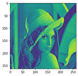
图像平滑
img = cv2.imread('lenaNoise.png')

cv2.imshow('img', img)
cv2.waitKey(0)
cv2.destroyAllWindows()

b,g,r = cv2.split(img)
img_rgb = cv2.merge((r,g,b))
plt.imshow(img_rgb)
plt.show()

# 均值滤波
# 简单的平均卷积操作
blur = cv2.blur(img, (3, 3))

cv2.imshow('blur', blur)
cv2.waitKey(0)
cv2.destroyAllWindows()

b,g,r = cv2.split(blur)
blur_rgb = cv2.merge((r,g,b))
plt.imshow(blur_rgb)
plt.show()

# 方框滤波
# 基本和均值一样,可以选择归一化
box = cv2.boxFilter(img,-1,(3,3), normalize=True)  #-1表示颜色通道数与之前输入的图像颜色通道数一致

cv2.imshow('box', box)
cv2.waitKey(0)
cv2.destroyAllWindows()

b,g,r = cv2.split(box)
box_rgb = cv2.merge((r,g,b))
plt.imshow(box_rgb)
plt.show()
# 方框滤波
# 基本和均值一样,可以选择归一化,容易越界 ,即像素值大于255
box = cv2.boxFilter(img,-1,(3,3), normalize=False)

cv2.imshow('box', box)
cv2.waitKey(0)
cv2.destroyAllWindows()

b,g,r = cv2.split(box)
box_rgb = cv2.merge((r,g,b))
plt.imshow(box_rgb)
plt.show()

# 高斯滤波
# 高斯模糊的卷积核里的数值是满足高斯分布,相当于更重视中间的,即核中间像素值的权重比较大
aussian = cv2.GaussianBlur(img, (5, 5), 1)

cv2.imshow('aussian', aussian)
cv2.waitKey(0)
cv2.destroyAllWindows()

b,g,r = cv2.split(aussian)
aussian_rgb = cv2.merge((r,g,b))
plt.imshow(aussian_rgb)
plt.show()

# 中值滤波
# 相当于用中值代替
median = cv2.medianBlur(img, 5)  # 中值滤波

cv2.imshow('median', median)
cv2.waitKey(0)
cv2.destroyAllWindows()

b,g,r = cv2.split(median)
median_rgb = cv2.merge((r,g,b))
plt.imshow(median_rgb)
plt.show()

# 展示所有的
res = np.hstack((blur,aussian,median)) #横着拼接在一起
#res = np.vstack((blur,aussian,median)) #竖着拼接在一起
#print (res)
cv2.imshow('median vs average', res)
cv2.waitKey(0)
cv2.destroyAllWindows()

b,g,r = cv2.split(res)
res_rgb = cv2.merge((r,g,b))
plt.imshow(res_rgb)
plt.show()

形态学-腐蚀操作
img = cv2.imread('cloudytosunny1.png')

cv2.imshow('img', img)
cv2.waitKey(0)
cv2.destroyAllWindows()

b,g,r = cv2.split(img)
img_rgb = cv2.merge((r,g,b))
plt.imshow(img_rgb)
plt.show()

kernel = np.ones((4,4),np.uint8)
erosion = cv2.erode(img,kernel,iterations = 1)

cv2.imshow('erosion', erosion)
cv2.waitKey(0)
cv2.destroyAllWindows()

b,g,r = cv2.split(erosion)
erosion_rgb = cv2.merge((r,g,b))
plt.imshow(erosion_rgb)
plt.show()

pie = cv2.imread('pie.png')

cv2.imshow('pie', pie)
cv2.waitKey(0)
cv2.destroyAllWindows()

b,g,r = cv2.split(pie)
pie_rgb = cv2.merge((r,g,b))
plt.imshow(pie_rgb)
plt.show()

kernel = np.ones((30,30),np.uint8)
erosion_1 = cv2.erode(pie,kernel,iterations = 1)
erosion_2 = cv2.erode(pie,kernel,iterations = 2)
erosion_3 = cv2.erode(pie,kernel,iterations = 3)
res = np.hstack((erosion_1,erosion_2,erosion_3))
cv2.imshow('res', res)
cv2.waitKey(0)
cv2.destroyAllWindows()

b,g,r = cv2.split(res)
res_rgb = cv2.merge((r,g,b))
plt.imshow(res_rgb)
plt.show()

形态学-膨胀操作
img = cv2.imread('cloudytosunny1.png')
cv2.imshow('img', img)
cv2.waitKey(0)
cv2.destroyAllWindows()

b,g,r = cv2.split(img)
img_rgb = cv2.merge((r,g,b))
plt.imshow(img_rgb)
plt.show()
kernel = np.ones((5,5),np.uint8)
sunny_erosion = cv2.erode(img,kernel,iterations = 1)

cv2.imshow('erosion', sunny_erosion)
cv2.waitKey(0)
cv2.destroyAllWindows()

b,g,r = cv2.split(sunny_erosion)
sunny_erosion_rgb = cv2.merge((r,g,b))
plt.imshow(sunny_erosion_rgb)
plt.show()

kernel = np.ones((5,5),np.uint8)
sunny_dilate = cv2.dilate(sunny_erosion,kernel,iterations = 1)

cv2.imshow('dilate', sunny_dilate)
cv2.waitKey(0)
cv2.destroyAllWindows()

b,g,r = cv2.split(sunny_dilate)
sunny_dilate_rgb = cv2.merge((r,g,b))
plt.imshow(sunny_dilate_rgb)
plt.show()

pie = cv2.imread('pie.png')

kernel = np.ones((30,30),np.uint8)
dilate_1 = cv2.dilate(pie,kernel,iterations = 1)
dilate_2 = cv2.dilate(pie,kernel,iterations = 2)
dilate_3 = cv2.dilate(pie,kernel,iterations = 3)
res = np.hstack((dilate_1,dilate_2,dilate_3))
cv2.imshow('res', res)
cv2.waitKey(0)
cv2.destroyAllWindows()

b,g,r = cv2.split(res)
res_rgb = cv2.merge((r,g,b))
plt.imshow(res_rgb)
plt.show()

开运算与闭运算
# 开:先腐蚀,再膨胀
img = cv2.imread('cloudytosunny1.png')

kernel = np.ones((5,5),np.uint8)
opening = cv2.morphologyEx(img, cv2.MORPH_OPEN, kernel)

cv2.imshow('opening', opening)
cv2.waitKey(0)
cv2.destroyAllWindows()

b,g,r = cv2.split(opening)
opening_rgb = cv2.merge((r,g,b))
plt.imshow(opening_rgb)
plt.show()
# 闭:先膨胀,再腐蚀
img = cv2.imread('cloudytosunny1.png')

kernel = np.ones((5,5),np.uint8)
closing = cv2.morphologyEx(img, cv2.MORPH_CLOSE, kernel)

cv2.imshow('closing', closing)
cv2.waitKey(0)
cv2.destroyAllWindows()

b,g,r = cv2.split(closing)
closing_rgb = cv2.merge((r,g,b))
plt.imshow(closing_rgb)
plt.show()

梯度运算
# 梯度=膨胀-腐蚀
pie = cv2.imread('pie.png')
kernel = np.ones((7,7),np.uint8)
dilate = cv2.dilate(pie,kernel,iterations = 5)
erosion = cv2.erode(pie,kernel,iterations = 5)

res = np.hstack((dilate,erosion))

b,g,r = cv2.split(res)
res_rgb = cv2.merge((r,g,b))
plt.imshow(res_rgb)
plt.show()

gradient = cv2.morphologyEx(pie, cv2.MORPH_GRADIENT, kernel)

b,g,r = cv2.split(gradient)
gradient_rgb = cv2.merge((r,g,b))
plt.imshow(gradient_rgb)
plt.show()

礼帽与黑帽
- 礼帽 = 原始输入-开运算结果
- 黑帽 = 闭运算-原始输入
#礼帽
img = cv2.imread('cloudytosunny1.png')
tophat = cv2.morphologyEx(img, cv2.MORPH_TOPHAT, kernel)

b,g,r = cv2.split(tophat)
tophat_rgb = cv2.merge((r,g,b))
plt.imshow(tophat_rgb)
plt.show()

#黑帽
img = cv2.imread('cloudytosunny1.png')
blackhat  = cv2.morphologyEx(img,cv2.MORPH_BLACKHAT, kernel)

b,g,r = cv2.split(blackhat)
blackhat_rgb = cv2.merge((r,g,b))
plt.imshow(blackhat_rgb)
plt.show()

图像梯度-Sobel算子

img = cv2.imread('pie.png',cv2.IMREAD_GRAYSCALE)

# b,g,r = cv2.split(img)
# img_rgb = cv2.merge((r,g,b))
plt.imshow(img)
plt.show()

cv2.imshow("img",img)
cv2.waitKey()
cv2.destroyAllWindows()

dst = cv2.Sobel(src, ddepth, dx, dy, ksize)
- ddepth:图像的深度
- dx和dy分别表示水平和竖直方向
- ksize是Sobel算子的大小
def cv_show(img,name):
    b,g,r = cv2.split(img)
    img_rgb = cv2.merge((r,g,b))
    plt.imshow(img_rgb)
    plt.show()
def cv_show1(img,name):
    plt.imshow(img)
    plt.show()
    cv2.imshow(name,img)
    cv2.waitKey()
    cv2.destroyAllWindows()
sobelx = cv2.Sobel(img,cv2.CV_64F,1,0,ksize=3)

cv_show1(sobelx,'sobelx')

白到黑是正数,黑到白就是负数了,所有的负数会被截断成0,所以要取绝对值
sobelx = cv2.Sobel(img,cv2.CV_64F,1,0,ksize=3)
sobelx = cv2.convertScaleAbs(sobelx)
cv_show1(sobelx,'sobelx')

sobely = cv2.Sobel(img,cv2.CV_64F,0,1,ksize=3)
sobely = cv2.convertScaleAbs(sobely)
cv_show1(sobely,'sobely')

分别计算x和y,再求和
sobelxy = cv2.addWeighted(sobelx,0.5,sobely,0.5,0)
cv_show1(sobelxy,'sobelxy')

不建议直接计算
sobelxy=cv2.Sobel(img,cv2.CV_64F,1,1,ksize=3)
sobelxy = cv2.convertScaleAbs(sobelxy)
cv_show1(sobelxy,'sobelxy')

img = cv2.imread('lena.jpg',cv2.IMREAD_GRAYSCALE)
cv_show1(img,'img')
img = cv2.imread('lena.jpg',cv2.IMREAD_GRAYSCALE)
sobelx = cv2.Sobel(img,cv2.CV_64F,1,0,ksize=3)
sobelx = cv2.convertScaleAbs(sobelx)
sobely = cv2.Sobel(img,cv2.CV_64F,0,1,ksize=3)
sobely = cv2.convertScaleAbs(sobely)
sobelxy = cv2.addWeighted(sobelx,0.5,sobely,0.5,0)
cv_show1(sobelxy,'sobelxy')

img = cv2.imread(‘lena.jpg’,cv2.IMREAD_GRAYSCALE)
sobelxy=cv2.Sobel(img,cv2.CV_64F,1,1,ksize=3)
sobelxy = cv2.convertScaleAbs(sobelxy)
cv_show(sobelxy,‘sobelxy’)
图像梯度-Scharr算子

图像梯度-laplacian算子

#不同算子的差异
img = cv2.imread('lena.jpg',cv2.IMREAD_GRAYSCALE)
sobelx = cv2.Sobel(img,cv2.CV_64F,1,0,ksize=3)
sobely = cv2.Sobel(img,cv2.CV_64F,0,1,ksize=3)
sobelx = cv2.convertScaleAbs(sobelx)
sobely = cv2.convertScaleAbs(sobely)
sobelxy =  cv2.addWeighted(sobelx,0.5,sobely,0.5,0)

scharrx = cv2.Scharr(img,cv2.CV_64F,1,0)
scharry = cv2.Scharr(img,cv2.CV_64F,0,1)
scharrx = cv2.convertScaleAbs(scharrx)
scharry = cv2.convertScaleAbs(scharry)
scharrxy =  cv2.addWeighted(scharrx,0.5,scharry,0.5,0)

laplacian = cv2.Laplacian(img,cv2.CV_64F) #一般不会单独使用,会跟其他方法联合使用
laplacian = cv2.convertScaleAbs(laplacian)

res = np.hstack((sobelxy,scharrxy,laplacian))
cv_show1(res,'res')

img = cv2.imread('lena.jpg',cv2.IMREAD_GRAYSCALE)
cv_show1(img,'img')

Canny边缘检测
使用高斯滤波器,以平滑图像,滤除噪声。
计算图像中每个像素点的梯度强度和方向。
应用非极大值(Non-Maximum Suppression)抑制,以消除边缘检测带来的杂散响应。
应用双阈值(Double-Threshold)检测来确定真实的和潜在的边缘。
通过抑制孤立的弱边缘最终完成边缘检测。
1:高斯滤波器

2:梯度和方向

3:非极大值抑制


4:双阈值检测

img=cv2.imread("lena.jpg",cv2.IMREAD_GRAYSCALE)

v1=cv2.Canny(img,80,150)
v2=cv2.Canny(img,50,100)

res = np.hstack((v1,v2))
cv_show1(res,'res')

img=cv2.imread("car.png",cv2.IMREAD_GRAYSCALE)

v1=cv2.Canny(img,120,250)
v2=cv2.Canny(img,50,100)

res = np.hstack((v1,v2))
cv_show1(res,'res')

图像金字塔
- 高斯金字塔
- 拉普拉斯金字塔

高斯金字塔:向下采样方法(缩小)

高斯金字塔:向上采样方法(放大)

img=cv2.imread("AM.png")
cv_show(img,'img')
print (img.shape)

(442, 340, 3)
up=cv2.pyrUp(img)
cv_show(up,'up')
print (up.shape)

(884, 680, 3)
down=cv2.pyrDown(img)
cv_show(down,'down')
print (down.shape)

(221, 170, 3)
up2=cv2.pyrUp(up)
cv_show(up2,'up2')
print (up2.shape)

(1768, 1360, 3)
up=cv2.pyrUp(img)
up_down=cv2.pyrDown(up)
cv_show(up_down,'up_down')

cv_show(np.hstack((img,up_down)),'up_down')

up=cv2.pyrUp(img)
up_down=cv2.pyrDown(up)
cv_show(img-up_down,'img-up_down')

拉普拉斯金字塔

down=cv2.pyrDown(img)
down_up=cv2.pyrUp(down)
l_1=img-down_up
cv_show(l_1,'l_1')

图像轮廓
cv2.findContours(img,mode,method)
mode:轮廓检索模式
- RETR_EXTERNAL :只检索最外面的轮廓;
- RETR_LIST:检索所有的轮廓,并将其保存到一条链表当中;
- RETR_CCOMP:检索所有的轮廓,并将他们组织为两层:顶层是各部分的外部边界,第二层是空洞的边界;
- RETR_TREE:检索所有的轮廓,并重构嵌套轮廓的整个层次;
method:轮廓逼近方法
- CHAIN_APPROX_NONE:以Freeman链码的方式输出轮廓,所有其他方法输出多边形(顶点的序列)。
- CHAIN_APPROX_SIMPLE:压缩水平的、垂直的和斜的部分,也就是,函数只保留他们的终点部分。

为了更高的准确率,使用二值图像。
img = cv2.imread('contours.png')
gray = cv2.cvtColor(img, cv2.COLOR_BGR2GRAY)
ret, thresh = cv2.threshold(gray, 127, 255, cv2.THRESH_BINARY)
cv_show1(thresh,'thresh')

binary, contours, hierarchy = cv2.findContours(thresh, cv2.RETR_TREE, cv2.CHAIN_APPROX_NONE)
绘制轮廓
cv_show(img,'img')

#传入绘制图像,轮廓,轮廓索引,颜色模式,线条厚度
# 注意需要copy,要不原图会变。。。
draw_img = img.copy()
res = cv2.drawContours(draw_img, contours, -1, (0, 0, 255), 2)
cv_show(res,'res')

draw_img = img.copy()
res = cv2.drawContours(draw_img, contours, 0, (0, 0, 255), 2)
cv_show(res,'res')

轮廓特征
cnt = contours[0]
#面积
cv2.contourArea(cnt)
8500.5
#周长,True表示闭合的
cv2.arcLength(cnt,True)
437.9482651948929
轮廓近似

img = cv2.imread('contours2.png')

gray = cv2.cvtColor(img, cv2.COLOR_BGR2GRAY)
ret, thresh = cv2.threshold(gray, 127, 255, cv2.THRESH_BINARY)
binary, contours, hierarchy = cv2.findContours(thresh, cv2.RETR_TREE, cv2.CHAIN_APPROX_NONE)
cnt = contours[0]

draw_img = img.copy()
res = cv2.drawContours(draw_img, [cnt], -1, (0, 0, 255), 2)
cv_show(res,'res')

epsilon = 0.1*cv2.arcLength(cnt,True)
approx = cv2.approxPolyDP(cnt,epsilon,True)

draw_img = img.copy()
res = cv2.drawContours(draw_img, [approx], -1, (0, 0, 255), 2)
cv_show(res,'res')

边界矩形
img = cv2.imread('contours.png')

gray = cv2.cvtColor(img, cv2.COLOR_BGR2GRAY)
ret, thresh = cv2.threshold(gray, 127, 255, cv2.THRESH_BINARY)
binary, contours, hierarchy = cv2.findContours(thresh, cv2.RETR_TREE, cv2.CHAIN_APPROX_NONE)
cnt = contours[0]

x,y,w,h = cv2.boundingRect(cnt)
img = cv2.rectangle(img,(x,y),(x+w,y+h),(0,255,0),2)
cv_show(img,'img')

area = cv2.contourArea(cnt)
x, y, w, h = cv2.boundingRect(cnt)
rect_area = w * h
extent = float(area) / rect_area
print ('轮廓面积与边界矩形比',extent)
轮廓面积与边界矩形比 0.5154317244724715
外接圆
(x,y),radius = cv2.minEnclosingCircle(cnt)
center = (int(x),int(y))
radius = int(radius)
img = cv2.circle(img,center,radius,(0,255,0),2)
cv_show(img,'img')

傅里叶变换
我们生活在时间的世界中,早上7:00起来吃早饭,8:00去挤地铁,9:00开始上班。。。以时间为参照就是时域分析。
但是在频域中一切都是静止的!
https://zhuanlan.zhihu.com/p/19763358
傅里叶变换的作用
高频:变化剧烈的灰度分量,例如边界
低频:变化缓慢的灰度分量,例如一片大海
滤波
低通滤波器:只保留低频,会使得图像模糊
高通滤波器:只保留高频,会使得图像细节增强
opencv中主要就是cv2.dft()和cv2.idft(),输入图像需要先转换成np.float32 格式。
得到的结果中频率为0的部分会在左上角,通常要转换到中心位置,可以通过shift变换来实现。
cv2.dft()返回的结果是双通道的(实部,虚部),通常还需要转换成图像格式才能展示(0,255)。
import numpy as np
import cv2
from matplotlib import pyplot as plt

img = cv2.imread('lena.jpg',0)

img_float32 = np.float32(img)

dft = cv2.dft(img_float32, flags = cv2.DFT_COMPLEX_OUTPUT)
dft_shift = np.fft.fftshift(dft)
# 得到灰度图能表示的形式
magnitude_spectrum = 20*np.log(cv2.magnitude(dft_shift[:,:,0],dft_shift[:,:,1]))

plt.subplot(121),plt.imshow(img, cmap = 'gray')
plt.title('Input Image'), plt.xticks([]), plt.yticks([])
plt.subplot(122),plt.imshow(magnitude_spectrum, cmap = 'gray')
plt.title('Magnitude Spectrum'), plt.xticks([]), plt.yticks([])
plt.show()

import numpy as np
import cv2
from matplotlib import pyplot as plt

img = cv2.imread('lena.jpg',0)

img_float32 = np.float32(img)

dft = cv2.dft(img_float32, flags = cv2.DFT_COMPLEX_OUTPUT)
dft_shift = np.fft.fftshift(dft)

rows, cols = img.shape
crow, ccol = int(rows/2) , int(cols/2)     # 中心位置

# 低通滤波
mask = np.zeros((rows, cols, 2), np.uint8)
mask[crow-30:crow+30, ccol-30:ccol+30] = 1

# IDFT
fshift = dft_shift*mask
f_ishift = np.fft.ifftshift(fshift)
img_back = cv2.idft(f_ishift)
img_back = cv2.magnitude(img_back[:,:,0],img_back[:,:,1])

plt.subplot(121),plt.imshow(img, cmap = 'gray')
plt.title('Input Image'), plt.xticks([]), plt.yticks([])
plt.subplot(122),plt.imshow(img_back, cmap = 'gray')
plt.title('Result'), plt.xticks([]), plt.yticks([])

plt.show()

img = cv2.imread('lena.jpg',0)

img_float32 = np.float32(img)

dft = cv2.dft(img_float32, flags = cv2.DFT_COMPLEX_OUTPUT)
dft_shift = np.fft.fftshift(dft)

rows, cols = img.shape
crow, ccol = int(rows/2) , int(cols/2)     # 中心位置

# 高通滤波
mask = np.ones((rows, cols, 2), np.uint8)
mask[crow-30:crow+30, ccol-30:ccol+30] = 0

# IDFT
fshift = dft_shift*mask
f_ishift = np.fft.ifftshift(fshift)
img_back = cv2.idft(f_ishift)
img_back = cv2.magnitude(img_back[:,:,0],img_back[:,:,1])

plt.subplot(121),plt.imshow(img, cmap = 'gray')
plt.title('Input Image'), plt.xticks([]), plt.yticks([])
plt.subplot(122),plt.imshow(img_back, cmap = 'gray')
plt.title('Result'), plt.xticks([]), plt.yticks([])

plt.show()

边栏推荐
- Crawler case 1: JS reversely obtains HD Wallpapers of minimalist Wallpapers
- Pic 10B parsing
- Esp8266wifi module tutorial: punctual atom atk-esp8266 for network communication, single chip microcomputer and computer, single chip microcomputer and mobile phone to send data
- Comparison between Apple Wireless charging scheme and 5W wireless charging scheme
- h5 localStorage
- Go语言浅拷贝与深拷贝
- Reflection example of ads2020 simulation signal
- "System error 5 occurred when win10 started mysql. Access denied"
- golang json unsupported value: NaN 处理
- Bluebridge cup 1 introduction training Fibonacci series
猜你喜欢

(1) Turn on the LED

Uniapp uses uviewui

Discrete device ~ diode triode
![[postgraduate entrance examination] group planning: interrupted](/img/ec/1f3dc0ac22e3a80d721303864d2337.jpg)
[postgraduate entrance examination] group planning: interrupted

Introduction of laser drive circuit

Necessary protection ring for weak current detection

Cause analysis of serial communication overshoot and method of termination

Color code

Real machine debugging of uniapp custom base

Fabrication of modulation and demodulation circuit
随机推荐
Uploading pictures with FileReader object
Can the encrypted JS code and variable name be cracked and restored?
Database learning notes II
Common uniapp configurations
你为什么会浮躁
Recognize the interruption of 80s51
Getting started with idea
2020-10-20
[postgraduate entrance examination: planning group] clarify the relationship among memory, main memory, CPU, etc
h5 localStorage
optee中的timer代码导读
What if the service in Nacos cannot be deleted?
Delete dictionary from list
Relevant knowledge of DRF
(1) Turn on the LED
[issue 22] sheen cloud platform one side & two sides
Chapter VIII (classes and objects)
Mapping '/var/mobile/Library/Caches/com. apple. keyboards/images/tmp. gcyBAl37' failed: 'Invalid argume
Understanding of closures
XXL job configuration alarm email notification