当前位置:网站首页>[six articles talk about scalablegnn] around www 2022 best paper PASCA
[six articles talk about scalablegnn] around www 2022 best paper PASCA
2022-07-25 13:09:00 【chad_ lee】
Scalable GNN
《Simplifying Graph Convolutional Networks》 ICML 2019
《SIGN: Scalable Inception Graph Neural Networks》 ICML 2020 workshop
《Simple Spectral Graph Convolution》ICLR 2020
《Scalable and Adaptive Graph Neural Networks with Self-Label-Enhanced training》 arxiv’21 OGB Once the first place
《Graph Attention Multi-Layer Perceptron》 arxiv‘21 The same author
《PaSca: a Graph Neural Architecture Search System under the Scalable Paradigm》 WWW 2022 best paper
existing GNN The defects of
High Memory Cost
GNN Feature propagation operations in ( Neighbor aggregation mechanism 、 Message passing mechanism ) Involving the multiplication of a large sparse matrix and characteristic matrix , It takes more time ; If used during training GPU Speed up , Then we must put the matrix in GPU On the memory of , But this demand cannot be satisfied for the big picture . such as OGB The largest in the node classification dataset ogb The sparse adjacency matrix size of the dataset exceeds 50GB, At present, only 80GB Video memory version Tesla A100 To save , But you can use 250GB Memory operation , The latter is easier to get . So only distributed training GNN, But this will bring a lot
High Communication Cost
GNN Every feature propagation needs to aggregate neighbor features , about K Layer of GNN Come on , Each node needs to aggregate K Characteristics of neighbor nodes within hops , The number of nodes involved increases exponentially as the number of layers increases , This will bring a lot of communication overhead in distributed scenarios . For dense connected graphs , Each node almost needs to aggregate the node information of the whole graph every time it is trained . Some sampling algorithms (GraphSAGE) Can alleviate this problem , But because of the recursive neighbor aggregation mechanism in the training process , These algorithms still cause high communication costs .

It can be seen that the performance bottleneck is the communication overhead , Add GPU Can't effectively speed up training .
Inconsistent Receptive Field expansion speed

The receptive field expansion speed of different nodes is different , Therefore, the optimal receptive field of different nodes is also different . chart a Is random 20 Test results of nodes , use SGC( Only the first K Layer of feature) Experiments done , Record continuous operation 100 Proportion of predicted correct times in total times . It can be seen that the prediction accuracy of different nodes varies with the increase of feature propagation steps , Such as node 10, The number of propagation steps is 1 The maximum prediction accuracy is reached , Subsequently, the prediction accuracy decreased continuously ; And there are some nodes , Such as node 4, The prediction accuracy increases with the increase of feature propagation steps . Even if the trend is the same , The optimal convolution layers of different nodes are also different . Therefore, when the node characteristics of different propagation steps are weighted and summed , Different weights should be given .
Different tasks need to be designed separately GNN structure
The existing GNN Work is to design a model structure , In different mission scenarios ( Data sets ) Domain experts may be required to design specific model structures 、 The training process , Modeling costs are high .
Scalable GNN summary
The article first summarizes Scalable GNN Architectural paradigm .Sampling-based The method is not Scalable GNN, Because these models also need to aggregate neighbor nodes in the training process , Communication overhead cannot be avoided in distributed scenarios .
model decoupling
Some research points out that 【SGC】,GNN The performance of is mainly due to the feature propagation operation in each layer , Instead of nonlinear transformation operation . This gave birth to a series of decoupling GNN, They are designing GNN The feature propagation operation and nonlinear transformation operation are decoupled , All feature propagation operations are completed in advance during preprocessing , In model training, there is no need to spend time and effort to propagate features . therefore , In terms of scalability , As long as the sparse matrix and dense matrix multiplication in the feature propagation operation can be completed during preprocessing , The subsequent model training can be easily carried out on a single machine and a single card . Because the feature propagation operation is completed in the preprocessing process , Therefore, there is no need to use GPU Accelerate , You can use only CPU Perform matrix multiplication .
But these are decoupled GNN The specificity of different nodes was not distinguished during training .SIGN、S2GC、SAGN、GAMLP We consider specificity .
SGC—— Consider only the K Characteristics of the layer
《Simplifying Graph Convolutional Networks》 ICML‘19

In the pretreatment stage ,SGC use K-step Features obtained after feature propagation ( Only the first K Output of layer convolution ), As the initial feature of the node : X ‾ ← S K X \overline{\mathbf{X}} \leftarrow \mathbf{S}^{K} \mathbf{X} X←SKX, S \mathbf{S} S It's an adjacency matrix . Then only one is trained in the model training stage 1 Layer of MLP As a classifier .
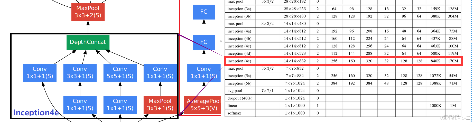
SIGN—— Consider different receptive fields
《SIGN: Scalable Inception Graph Neural Networks》 ICML‘20 workshop
SGC It only took K-step The obtained feature is used as the initial feature of the node , Obviously, it is not optimal for all nodes ,SIGN take 0~K-step All the features are stitched together , It retains the characteristics of all receptive fields :
Z = σ ( [ X Θ 0 , A 1 X Θ 1 , … , A r X Θ r ] ) Y = ξ ( Z Ω ) \begin{aligned} \mathbf{Z} &=\sigma\left(\left[\mathbf{X} \boldsymbol{\Theta}_{0}, \mathbf{A}_{1} \mathbf{X} \boldsymbol{\Theta}_{1}, \ldots, \mathbf{A}_{r} \mathbf{X} \boldsymbol{\Theta}_{r}\right]\right) \\ \mathbf{Y} &=\xi(\mathbf{Z} \boldsymbol{\Omega}) \end{aligned} ZY=σ([XΘ0,A1XΘ1,…,ArXΘr])=ξ(ZΩ)
Θ \boldsymbol{\Theta} Θ and Ω \boldsymbol{\Omega} Ω All training parameters . The disadvantage is that the space cost of splicing is directly proportional to the number of convolution layers .
S2GC——PPR+ Average
《Simple Spectral Graph Convolution》ICLR‘20

Y ^ = softmax ( 1 K ∑ k = 1 K ( ( 1 − α ) T ~ k X + α X ) W ) \hat{Y}=\operatorname{softmax}\left(\frac{1}{K} \sum_{k=1}^{K}\left((1-\alpha) \tilde{\mathbf{T}}^{k} \mathbf{X}+\alpha \mathbf{X}\right) \mathbf{W}\right) Y^=softmax(K1k=1∑K((1−α)T~kX+αX)W)
T T T Or adjacency matrix ,S2GC In fact, it is approximate in probability ( 1 − α 1-\alpha 1−α) Rebooted PPR Get the characteristics of each layer , And then add them evenly , As the initial feature of the node .
SAGN—— Different receptive fields attention Sum up
《Scalable and Adaptive Graph Neural Networks with Self-Label-Enhanced training》 arxiv’21

hold SIGN The splicing operation in is replaced by attention Weighted sum of , Weighted sum of different receptive field characteristics , Later articles are follow This paradigm .
GAMLP—— Design attention
《Graph Attention Multi-Layer Perceptron》 arxiv‘21

1、Smoothing Attention
It can be understood as the node feature after infinite times of feature propagation X i ( ∞ ) X_{i}^{(\infty)} Xi(∞) As reference vector , And then calculate attention:
X ~ i ( l ) = X i ( l ) ∥ X i ( ∞ ) , w ~ i ( l ) = δ ( X ~ i ( l ) ⋅ s ) , w i ( l ) = e w ~ i ( l ) / ∑ k = 0 K e w ~ i ( k ) \widetilde{\mathbf{X}}_{i}^{(l)}=\mathbf{X}_{i}^{(l)} \| \mathbf{X}_{i}^{(\infty)}, \quad \widetilde{w}_{i}(l)=\delta\left(\tilde{\mathbf{X}}_{i}^{(l)} \cdot s\right), \quad w_{i}(l)=e^{\widetilde{w}_{i}(l)} / \sum_{k=0}^{K} e^{\widetilde{w}_{i}(k)} Xi(l)=Xi(l)∥Xi(∞),wi(l)=δ(X~i(l)⋅s),wi(l)=ewi(l)/k=0∑Kewi(k)
among s ∈ R 1 × d s \in \mathbb{R}^{1 \times d} s∈R1×d It's a trainable parameter . The larger w i ( l ) w_{i}(l) wi(l) It means that nodes v i v_{i} vi Of l-step The propagation characteristics are far away from the infinite propagation state , The risk of becoming noise is small . With larger w i ( l ) w_{i}(l) wi(l) The transmission characteristics of should contribute more to the combination of characteristics .
2、Recursive Attention
Recursively calculate the information gain in the process of feature propagation :
X ~ i ( l ) = X i ( l ) ∥ ∑ k = 0 l − 1 w i ( k ) X i ( k ) , w ~ i ( l ) = δ ( X ~ i ( l ) ⋅ s ) , w i ( l ) = e w ~ i ( l ) / ∑ k = 0 K e w ~ i ( k ) \tilde{\mathbf{X}}_{i}^{(l)}=\mathbf{X}_{i}^{(l)} \| \sum_{k=0}^{l-1} w_{i}(k) \mathbf{X}_{i}^{(k)}, \tilde{w}_{i}(l)=\delta\left(\tilde{\mathbf{X}}_{i}^{(l)} \cdot s\right), w_{i}(l)=e^{\tilde{w}_{i}(l)} / \sum_{k=0}^{K} e^{\tilde{w}_{i}(k)} X~i(l)=Xi(l)∥∑k=0l−1wi(k)Xi(k),w~i(l)=δ(X~i(l)⋅s),wi(l)=ew~i(l)/∑k=0Kew~i(k)
The larger w i ( l ) w_{i}(l) wi(l) Signifying characteristics X i ( l ) \mathbf{X}_{i}^{(l)} Xi(l) Yes v i v_{i} vi The current state of is more important ( Compared with the previous layer, the combination features account for a higher proportion ).
3、JK Attention

Will all step Feature input to MLP,MLP The output result is used as the reference vector , Calculation attention:
X ~ i ( l ) = X i ( l ) ∥ E i , w ~ i ( l ) = δ ( X ~ i ( l ) ⋅ s ) , w i ( l ) = e w ~ i ( l ) / ∑ k = 0 K e w ~ i ( k ) E i = M L P ( X i ( 1 ) ∥ X i ( 2 ) ∥ … ∥ X i ( K ) ) \tilde{X}_{i}^{(l)}=X_{i}^{(l)} \| E_{i}, \quad \widetilde{w}_{i}(l)=\delta\left(\tilde{X}_{i}^{(l)} \cdot \mathrm{s}\right), \quad w_{\mathrm{i}}(l)=e^{\widetilde{w}_{i}(l)} / \sum_{k=0}^{K} e^{\widetilde{w}_{i}(k)} \\ \mathbf{E}_{i}=\mathbf{M L P}\left(\mathbf{X}_{i}^{(1)}\left\|\mathbf{X}_{i}^{(2)}\right\| \ldots \| \mathbf{X}_{i}^{(K)}\right) X~i(l)=Xi(l)∥Ei,wi(l)=δ(X~i(l)⋅s),wi(l)=ewi(l)/k=0∑Kewi(k)Ei=MLP(Xi(1)∥∥Xi(2)∥∥…∥Xi(K))
Scalable GNN Model design space
《PaSca: a Graph Neural Architecture Search System under the Scalable Paradigm》 WWW 2022 best paper
As mentioned above Scalable GNN Are a specific model architecture , According to the above work , It can be concluded that Scalable GNN Model design space , Then you can define the search target ( Accuracy and speed ), Search for the one that is suitable for the current task scenario Scalable GNN.

Scalable GNN The model design of can be divided into three stages :
1、 Pretreatment stage
Aggregation step( K p r e K_{pre} Kpre) It refers to the feature obtained by convolution of several layers at most .
Graph aggregator( G A p r e GA_{pre} GApre) It refers to the adjacency matrix used by the neighbor aggregation mechanism , For example, after standardization A、PPR etc. .
It's described above SGC、SIGN、SAGN、GAMLP It's used A;S2GC It's using PPR.
2、 Model training stage
Message aggregators( M A MA MA) It refers to how to use the obtained k-steps Characteristics of .None Only the last layer (SGC);Mean Namely S2GC;Concatenate Namely SIGN;Weighted Namely SAGN;Adaptive Namely GAMLP. It's not good to use only one layer , Because different nodes have different optimal receptive fields .
Transformation step( K t r a n s K_{trans} Ktrans) Refer to MLP The number of layers .
3、 Post processing stage
there K p o s K_{pos} Kpos and G A p o s t GA_{post} GApost And pretreatment stage K p r e K_{pre} Kpre and G A p r e GA_{pre} GApre identical , The purpose is to Label Propagation, The model predicts Classification probability distribution Spread it several times , Be similar to APPNP, But it is directly transmitted to the model output after training .

The whole model design space contains 18 Ten thousand model architectures , The above summary Scalable GNN Are concrete examples of this design space :
Model structure automatic search system ( Auto search super parameter )

This part of the article is very short . It is divided into two engines : One is the search engine , One is the evaluation engine .
Search engine is based on Bayesian optimization to realize the recommendation of model structure . First, define the optimization objective : Accuracy and training speed . Then model the relationship between the observed model structure and the optimization goal ( Try to establish a mapping ), Return a model structure that can balance multiple optimization objectives , Let the evaluation engine verify .
The evaluation engine is to train the model , Then return the results to the search engine , In this way, there is another observation result of search engine .
experimental result
Communication overhead

Model accuracy and efficiency :

PaSca The found model can better balance the training efficiency and model accuracy . It can be seen from the right figure that there is no decoupling GCN Compared with decoupling GCN, Performance has no significant advantage , But the efficiency is more than 100 times worse .

ScalableGNN No, over-smoothing, Because the output of deep convolution is used as an initial feature ,Attention You can pay attention or not .
边栏推荐
- Can flinkcdc import multiple tables in mongodb database together?
- Detailed explanation of the training and prediction process of deep learning [taking lenet model and cifar10 data set as examples]
- 程序员成长第二十七篇:如何评估需求优先级?
- 7行代码让B站崩溃3小时,竟因“一个诡计多端的0”
- The larger the convolution kernel, the stronger the performance? An interpretation of replknet model
- 网络空间安全 渗透攻防9(PKI)
- 2022.07.24 (lc_6126_design food scoring system)
- A turbulent life
- EMQX Cloud 更新:日志分析增加更多参数,监控运维更省心
- 牛客论坛项目部署总结
猜你喜欢
![[problem solving] ibatis.binding BindingException: Type interface xxDao is not known to the MapperRegistry.](/img/00/65eaad4e05089a0f8c199786766396.png)
[problem solving] ibatis.binding BindingException: Type interface xxDao is not known to the MapperRegistry.

【AI4Code】《Unified Pre-training for Program Understanding and Generation》 NAACL 2021

Date and time function of MySQL function summary

Convolutional neural network model -- vgg-16 network structure and code implementation
卷积神经网络模型之——GoogLeNet网络结构与代码实现
![[today in history] July 25: IBM obtained the first patent; Verizon acquires Yahoo; Amazon releases fire phone](/img/f6/d422367483542a0351923f2df27347.jpg)
[today in history] July 25: IBM obtained the first patent; Verizon acquires Yahoo; Amazon releases fire phone
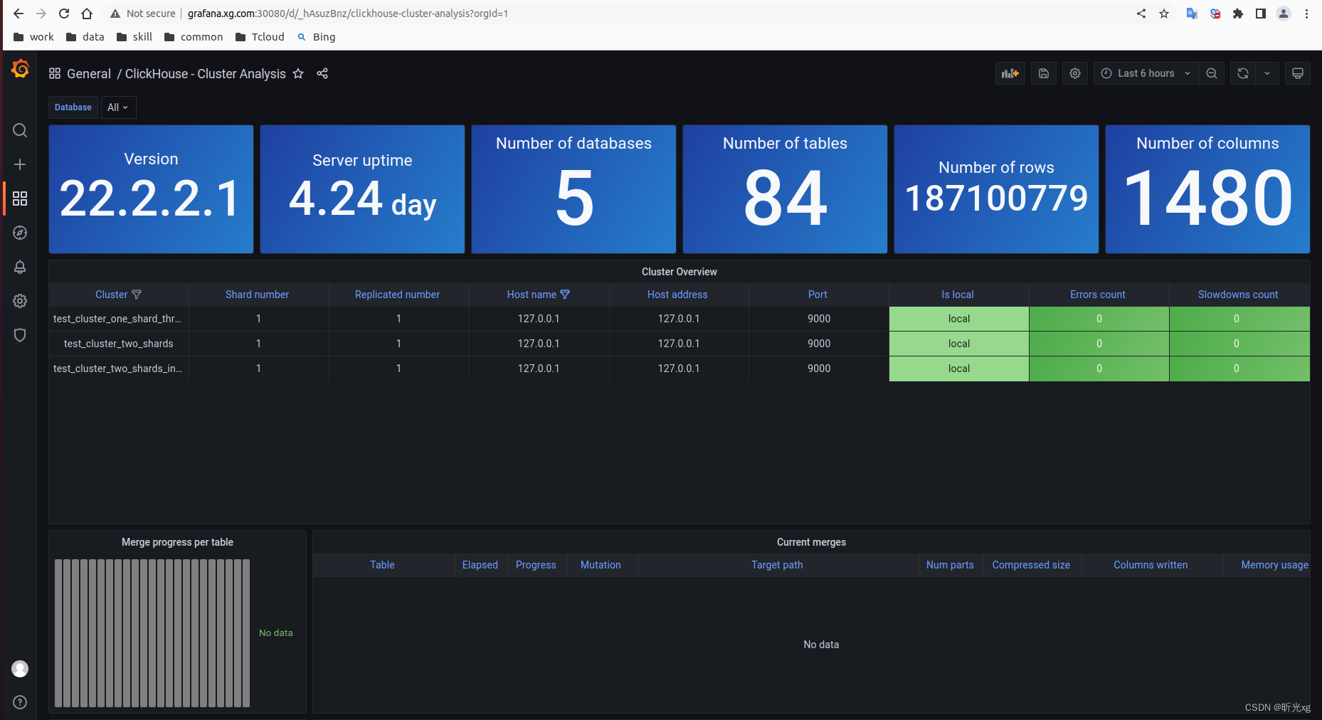
clickhouse笔记03-- Grafana 接入ClickHouse

零基础学习CANoe Panel(15)—— 文本输出(CAPL Output View )

Shell common script: judge whether the file of the remote host exists

Introduction to web security UDP testing and defense
随机推荐
录制和剪辑视频,如何解决占用空间过大的问题?
EMQX Cloud 更新:日志分析增加更多参数,监控运维更省心
VIM tip: always show line numbers
Detailed explanation of the training and prediction process of deep learning [taking lenet model and cifar10 data set as examples]
Convolutional neural network model -- alexnet network structure and code implementation
Cv2.resize function reports an error: error: (-215:assertion failed) func= 0 in function ‘cv::hal::resize‘
Convolutional neural network model -- lenet network structure and code implementation
Shell常用脚本:检测某域名、IP地址是否通
R language GLM generalized linear model: logistic regression, Poisson regression fitting mouse clinical trial data (dose and response) examples and self-test questions
Vim技巧:永远显示行号
Chapter5 : Deep Learning and Computational Chemistry
Convolutional neural network model -- vgg-16 network structure and code implementation
yum和vim须掌握的常用操作
【AI4Code】《InferCode: Self-Supervised Learning of Code Representations by Predicting Subtrees》ICSE‘21
[Video] Markov chain Monte Carlo method MCMC principle and R language implementation | data sharing
2022.07.24 (lc_6124_the first letter that appears twice)
OAuth, JWT, oidc, you mess me up
[operation and maintenance, implementation of high-quality products] interview skills for technical positions with a monthly salary of 10k+
Oran special series-21: major players (equipment manufacturers) and their respective attitudes and areas of expertise
Atcoder beginer contest 261 f / / tree array