当前位置：网站首页>Pymoo learning (3): use multi-objective optimization to find the set of optimal solutions

Pymoo learning (3): use multi-objective optimization to find the set of optimal solutions

2022-07-23 17:21:00 【Inji】

List of articles

1 Bi objective optimization
2 Python solve
3 Complete code

1 Bi objective optimization

It is shown as follows ：
$\begin{aligned} \min & f_{1}(x)=100\left(x_{1}^{2}+x_{2}^{2}\right) \\ \max & f_{2}(x)=-\left(x_{1}-1\right)^{2}-x_{2}^{2} \\ \text { s.t. } & g_{1}(x)=2\left(x_{1}-0.1\right)\left(x_{1}-0.9\right) \leq 0 \\ & g_{2}(x)=20\left(x_{1}-0.4\right)\left(x_{1}-0.6\right) \geq 0 \\ &-2 \leq x_{1} \leq 2 \\ &-2 \leq x_{2} \leq 2 \\ & x \in \mathbb{R} \end{aligned}$ First, it needs to be transformed into the standard form of optimization problem ：
1） $f_2(x)$ Replace $f_2(x)$ ;
2） Inequality constraints are converted to $\leq0$ In the form of , namely $-g_2(x)\leq0$ ;
3） Normalized variable , Make it equal in importance , namely $g_1(x)/(2*(-0.1)*(-0.9))$ , $g_2(x)/(20*(-0.4)*(-0.6))$ . The conversion result is as follows ：
$\begin{aligned} \min & f_{1}(x)=100\left(x_{1}^{2}+x_{2}^{2}\right) \\ \min & f_{2}(x)=\left(x_{1}-1\right)^{2}+x_{2}^{2} \\ \text { s.t. } & g_{1}(x)=2\left(x_{1}-0.1\right)\left(x_{1}-0.9\right)/0.18 \leq 0 \\ & g_{2}(x)=-20\left(x_{1}-0.4\right)\left(x_{1}-0.6\right)/4.8 \leq 0 \\ &-2 \leq x_{1} \leq 2 \\ &-2 \leq x_{2} \leq 2 \\ & x \in \mathbb{R} \end{aligned}$

2 Python solve

This section uses element-wise solve , It is one of the three solutions ：

import numpy as np
from pymoo.core.problem import ElementwiseProblem


class MyProblem(ElementwiseProblem):

    def __init__(self):
        super(MyProblem, self).__init__(
            n_var=2,  #  Number of variables 
            n_obj=2,  #  Number of optimization objectives 
            n_constr=2,  #  Number of constraints 
            xl=np.array([-2, -2]),  #  Lower bound of variable 
            xu=np.array([2, 2])  #  The upper limit of the variable 
        )

    def _evaluate(self, x, out, *args, **kwargs):
        """ :param x: 1D vector , The length is n_var :param out: :param args: :param kwargs: :return: """
        #  Objective function 
        f1 = 100 * (x[0]**2 + x[1]**2)
        f2 = (x[0] - 1)**2 + x[1]**2

        #  constraint condition 
        g1 = 2 * (x[0] - 0.1) * (x[0] - 0.9) / 0.18
        g2 = - 20 * (x[0] - 0.4) * (x[0] - 0.6) / 4.8

        #  Store the target value and constraint value 
        out["F"] = [f1, f2]
        out["G"] = [g1, g2]

notes ： The three ways to solve the problem are as follows ：
1）element-wise： Every time $x$ call _evaluate;
2）vectorized： $x$ Represents a set of solutions ;
3）functional： Provide each goal and constraint as a function .

2.1 initialization

The optimization problem in the diagram is very simple , There are only two goals and two constraints , The following is the famous multi-objective Algorithm NSGA-II The initialization ：

from pymoo.algorithms.moo.nsga2 import NSGA2
from pymoo.factory import get_sampling, get_crossover, get_mutation


algorithm = NSGA2(
    pop_size=40,  #  Population number 
    n_offsprings=10,  #  The number of offspring 
    sampling=get_sampling("real_random"),  #  The way of sampling , Such as random sampling 
    crossover=get_crossover("real_sbx", prob=0.9, eta=15),  #  mating system  , Such as analog binary 
    mutation=get_mutation("real_pm", eta=20),  #  The way of variation , Polynomial variation 
    eliminate_duplicates=True   #  Ensure that the target values of future generations are different 
)

2.2 Termination conditions

Before optimization, you need to define Termination conditions . Common methods include ：
1） Limit the total number of function evaluations ;
2） Limit the number of iterations of the algorithm ;
3） customized ： Some algorithms implement their own termination conditions , For example, when simplex degenerates Nelder-Mead Or use supplier library CMA-ES.
Because this example is relatively simple , Use 40 Iterations as the termination condition ：

from pymoo.factory import get_termination

termination = get_termination("n_gen", 40)

2.3 Optimize

The minimization method is as follows ：

from pymoo.optimize import minimize

res = minimize(
    problem=MyProblem(),
    algorithm=algorithm,
    termination=termination,
    seed=1,
    save_history=True,
    verbose=True    #  Output control variables 
)

#  Store feasible solutions 
X = res.X
#  Store the target value 
F = res.F

Output is as follows , Each column represents ：
1） The number of iterations ;
2） Number of evaluations ;
3） Overall minimum constraint violation ;
4） Overall average constraint violation ;
5） The number of non dominant solutions ;
6） and 7） Search for motion related indicators in space .

=====================================================================================
n_gen |  n_eval |   cv (min)   |   cv (avg)   |  n_nds  |     eps      |  indicator  
=====================================================================================
    1 |      40 |  0.00000E+00 |  2.36399E+01 |       1 |            - |            -
    2 |      50 |  0.00000E+00 |  1.15486E+01 |       1 |  0.00000E+00 |            f
    3 |      60 |  0.00000E+00 |  5.277918607 |       1 |  0.00000E+00 |            f
    4 |      70 |  0.00000E+00 |  2.406068542 |       2 |  1.000000000 |        ideal
    5 |      80 |  0.00000E+00 |  0.908316880 |       3 |  0.869706146 |        ideal
    6 |      90 |  0.00000E+00 |  0.264746300 |       3 |  0.00000E+00 |            f
    7 |     100 |  0.00000E+00 |  0.054063822 |       4 |  0.023775686 |        ideal
    8 |     110 |  0.00000E+00 |  0.003060876 |       5 |  0.127815454 |        ideal
    9 |     120 |  0.00000E+00 |  0.00000E+00 |       6 |  0.085921728 |        ideal
   10 |     130 |  0.00000E+00 |  0.00000E+00 |       7 |  0.015715204 |            f
   11 |     140 |  0.00000E+00 |  0.00000E+00 |       8 |  0.015076323 |            f
   12 |     150 |  0.00000E+00 |  0.00000E+00 |       7 |  0.026135665 |            f
   13 |     160 |  0.00000E+00 |  0.00000E+00 |      10 |  0.010026699 |            f
   14 |     170 |  0.00000E+00 |  0.00000E+00 |      11 |  0.011833783 |            f
   15 |     180 |  0.00000E+00 |  0.00000E+00 |      12 |  0.008294035 |            f
   16 |     190 |  0.00000E+00 |  0.00000E+00 |      14 |  0.006095993 |        ideal
   17 |     200 |  0.00000E+00 |  0.00000E+00 |      17 |  0.002510398 |        ideal
   18 |     210 |  0.00000E+00 |  0.00000E+00 |      20 |  0.003652660 |            f
   19 |     220 |  0.00000E+00 |  0.00000E+00 |      20 |  0.010131820 |        nadir
   20 |     230 |  0.00000E+00 |  0.00000E+00 |      21 |  0.005676014 |            f
   21 |     240 |  0.00000E+00 |  0.00000E+00 |      25 |  0.010464402 |            f
   22 |     250 |  0.00000E+00 |  0.00000E+00 |      25 |  0.000547515 |            f
   23 |     260 |  0.00000E+00 |  0.00000E+00 |      28 |  0.001050255 |            f
   24 |     270 |  0.00000E+00 |  0.00000E+00 |      33 |  0.003841298 |            f
   25 |     280 |  0.00000E+00 |  0.00000E+00 |      37 |  0.006664377 |        nadir
   26 |     290 |  0.00000E+00 |  0.00000E+00 |      40 |  0.000963164 |            f
   27 |     300 |  0.00000E+00 |  0.00000E+00 |      40 |  0.000678243 |            f
   28 |     310 |  0.00000E+00 |  0.00000E+00 |      40 |  0.000815766 |            f
   29 |     320 |  0.00000E+00 |  0.00000E+00 |      40 |  0.001500814 |            f
   30 |     330 |  0.00000E+00 |  0.00000E+00 |      40 |  0.014706442 |        nadir
   31 |     340 |  0.00000E+00 |  0.00000E+00 |      40 |  0.003554320 |        ideal
   32 |     350 |  0.00000E+00 |  0.00000E+00 |      40 |  0.000624123 |            f
   33 |     360 |  0.00000E+00 |  0.00000E+00 |      40 |  0.000203925 |            f
   34 |     370 |  0.00000E+00 |  0.00000E+00 |      40 |  0.001048509 |            f
   35 |     380 |  0.00000E+00 |  0.00000E+00 |      40 |  0.001121103 |            f
   36 |     390 |  0.00000E+00 |  0.00000E+00 |      40 |  0.000664461 |            f
   37 |     400 |  0.00000E+00 |  0.00000E+00 |      40 |  0.000761066 |            f
   38 |     410 |  0.00000E+00 |  0.00000E+00 |      40 |  0.000521906 |            f
   39 |     420 |  0.00000E+00 |  0.00000E+00 |      40 |  0.004652095 |        nadir
   40 |     430 |  0.00000E+00 |  0.00000E+00 |      40 |  0.000287847 |            f

2.4 visualization

Visualization to better show the solution results ：

import matplotlib.pyplot as plt
problem = MyProblem()
xl, xu = problem.bounds()
plt.figure(figsize=(7, 5))
plt.scatter(X[:, 0], X[:, 1], s=30, facecolors='none', edgecolors='r')
plt.xlim(xl[0], xu[0])
plt.ylim(xl[1], xu[1])
plt.title("Search space")
plt.show()

plt.figure(figsize=(7, 5))
plt.scatter(F[:, 0], F[:, 1], s=30, facecolors='none', edgecolors='blue')
plt.title("Objective Space")
plt.show()

Output is as follows ：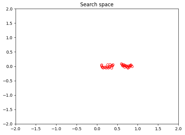

3 Complete code

import numpy as np
from pymoo.core.problem import ElementwiseProblem
from pymoo.algorithms.moo.nsga2 import NSGA2
from pymoo.factory import get_sampling, get_crossover, get_mutation
from pymoo.factory import get_termination
from pymoo.optimize import minimize


class MyProblem(ElementwiseProblem):

    def __init__(self):
        super(MyProblem, self).__init__(
            n_var=2,  #  Number of variables 
            n_obj=2,  #  Number of optimization objectives 
            n_constr=2,  #  Number of constraints 
            xl=np.array([-2, -2]),  #  Lower bound of variable 
            xu=np.array([2, 2])  #  The upper limit of the variable 
        )

    def _evaluate(self, x, out, *args, **kwargs):
        """ :param x: 1D vector , The length is n_var :param out: :param args: :param kwargs: :return: """
        #  Objective function 
        f1 = 100 * (x[0]**2 + x[1]**2)
        f2 = (x[0] - 1)**2 + x[1]**2

        #  constraint condition 
        g1 = 2 * (x[0] - 0.1) * (x[0] - 0.9) / 0.18
        g2 = - 20 * (x[0] - 0.4) * (x[0] - 0.6) / 4.8

        #  Store the target value and constraint value 
        out["F"] = [f1, f2]
        out["G"] = [g1, g2]


algorithm = NSGA2(
    pop_size=40,  #  Population number 
    n_offsprings=10,  #  The number of offspring 
    sampling=get_sampling("real_random"),  #  The way of sampling , Such as random sampling 
    crossover=get_crossover("real_sbx", prob=0.9, eta=15),  #  mating system  , Such as analog binary 
    mutation=get_mutation("real_pm", eta=20),  #  The way of variation , Polynomial variation 
    eliminate_duplicates=True   #  Ensure that the goals of future generations are different 
)

termination = get_termination("n_gen", 40)

res = minimize(
    problem=MyProblem(),
    algorithm=algorithm,
    termination=termination,
    seed=1,
    save_history=True,
    verbose=True    #  Output control variables 
)

#  Store feasible solutions 
X = res.X
#  Store the target value 
F = res.F

import matplotlib.pyplot as plt
problem = MyProblem()
xl, xu = problem.bounds()
plt.figure(figsize=(7, 5))
plt.scatter(X[:, 0], X[:, 1], s=30, facecolors='none', edgecolors='r')
plt.xlim(xl[0], xu[0])
plt.ylim(xl[1], xu[1])
plt.title("Search space")
plt.show()

plt.figure(figsize=(7, 5))
plt.scatter(F[:, 0], F[:, 1], s=30, facecolors='none', edgecolors='blue')
plt.title("Objective Space")
plt.show()