[on]learning dynamic and hierarchical traffic spatiotemporal features with transformer

Learning Dynamic and Hierarchical Traffic Spatiotemporal Features with Transformer

original text , see here
author ：Haoyang Yan, Xiaolei Ma
Periodical ：
keyword ：

Abstract

Traffic forecasting is an indispensable part of intelligent transportation system , Long term network wide accurate traffic speed prediction is one of the most challenging tasks . In recent years , Deep learning methods are becoming more and more popular in this field . Because traffic data is physically associated with the road network , Most of the proposed models regard it as a spatiotemporal graph modeling problem , And use graph based convolution network (GCN) Methods . These are based on GCN The model is highly dependent on a predefined and fixed adjacency matrix to reflect spatial dependencies . However , The predefined fixed adjacency matrix has limitations in reflecting the actual dependence of traffic flow . This paper proposes A new traffic transformer model , Used for spatio-temporal map modeling and long-term traffic forecasting , To overcome these limitations .Transformer It's natural language processing (NLP) The most popular framework in .Traffic Transformer Apply it to the space-time problem , The spatiotemporal features are extracted dynamically and hierarchically from the data through multiple heads' attention and masked multiple heads' attention mechanisms , And combine these features to predict traffic . Besides , Through analysis Attention weight matrix The influential parts of the road network can be found , So as to better understand the transportation network . The experimental results on the public transport network data set and the actual transport network data set show that , The performance of this model is better than the existing models .

1 Introduction

The urban transportation system meets the needs of passengers , Ensure the operation of the city . But with the accelerating process of Urbanization , Traffic congestion and other problems are becoming more and more difficult to solve . Intelligent transportation system can help alleviate traffic congestion , Traffic speed prediction is the basis of intelligent transportation system . Traffic speed is one of the most critical indicators to reflect traffic conditions . Many researchers have proposed different methods for traffic speed prediction , And achieved great success .

In recent years , Deep learning method It has been widely used in this field , It allows researchers to establish Data driven model To extract spatiotemporal features . Road network traffic flow data has two types of characteristics : Spatial and temporal characteristics . Time features can be extracted by different time series models , But there is no general method to extract spatial features . In limine , The researchers ignored the spatial features , Focus on a single path . Previous deep learning models usually transform traffic networks into grid like structures , And treat it as an image , utilize Convolutional neural networks (CNN) Extract spatial features . However , These transformations obviously lost a lot of information , And completely destroyed the network relationship . for example , Roads in the same grid are merged , Unable to analyze . Due to the physical association between traffic data and road network , The recently proposed model regards it as a spatiotemporal graph modeling problem , And use graph based convolution network (GCN) Methods . These are based on GCN The key of the model is the neighborhood matrix . Adjacency matrix defines the relationship between nodes and edges of a graph , This allows the model convolution to collect information from adjacent nodes . be based on gcn The model has achieved great success in the whole network traffic prediction . However , These are based on GCN There are still some limitations in our model .

️1.1 Limitations in GCN-based models

(a). It is difficult and expensive for human to define a perfect adjacency matrix . The adjacency matrix represents the messages delivered in the graph , But the propagation of traffic is complicated , Not simply based on distance , Some nodes can be viewed as abstract connections . for example , The sensors at the downtown intersection can represent the service level of the network to a certain extent . The sensor has a certain impact , Can be seen as abstractly connected to most sensors .

(b). The adjacent matrix is fixed in the model . Fixed adjacency matrix cannot handle week 、 Over the weekend 、 Morning peak 、 Dynamic flow under different conditions such as evening peak . Besides , Such as (a) Shown , There are inevitable errors in adjacent matrices . for example , At the intersection without left turn , The upstream and downstream sensors of the left turn route are close in space , But it is logically far away . A fixed neighborhood matrix means that these errors will always affect the model .

No depth or grade . The proposed model usually uses only one adjacent matrix . Some models use a set of adjacent matrices , But the results of these adjacent matrices are simply added or spliced . However , We have always wanted to use hierarchical “ depth ” Model .

In response to the above challenges , We found that spatial feature extraction and naturallanguageprocessing (NLP) There are similarities , And draw lessons from NLP It's an advanced way to .

1.2 Similarity between spatial feature extraction and NLP

Fig.1 The similarity between spatial feature extraction and naturallanguageprocessing .(a): Natural language data and traffic data can be regarded as sequential data ;(b): Changing the sequence will change the meaning ;(c): High dependencies can exist in sequences or even far away ;(d): Meaning is dynamic , And depends on other parts .

Spatial feature extraction and naturallanguageprocessing are not only similar in data features , And the challenges and difficulties are similar . Such as chart 1 (a) Shown , Both natural language data and traffic data can be regarded as sequential data . Natural language data is a sequence of words , Traffic data is a sequence of sensors . Such as chart 1 (b) Shown , Absolute and relative positions are important . Changing the order of the sequence will change the meaning . Such as chart 1 Shown , Long term dependence on NLP Very common in , Infer that tomorrow's date must go back to the beginning of the article . Each sensor in the traffic network can have an abstract impact on the sensor regardless of distance . Such as chart 1(d) Shown , Dependencies are dynamic , The meaning of a word depends on the context . Even the words in two sentences “it” It's exactly the same , The meaning of the two words is different . Again , The traffic status of the central node is the same , But the spatial dependencies of nodes are different .

Transformer The above challenges and difficulties have been solved , It has achieved great success in the field of naturallanguageprocessing , Is a robust sequence learning framework . Considering the similarity , This paper puts forward a kind of New traffic transformer model , be used for Spatiotemporal map modeling and long-term traffic forecasting , To overcome the problems based on GCN Limitations of the model . We will Transformer Applied to traffic forecasting problems . utilize Transformer Multiple attention mechanism , Dynamically extract the relationship between each pair of nodes through data . Stacking transformer layers allows our model to extract features hierarchically . Integrating features through attention mechanisms . stay Public transport network data set METR-LA And the experimental results on two real traffic network datasets generated by ourselves show that , The proposed model has better performance than the existing models . The main contributions of our work are summarized as follows :

• We propose a new traffic transformer model , Used for spatio-temporal map modeling and long-term traffic forecasting . It extracts and fuses the global and local spatial features of the whole network traffic flow , The prediction accuracy is significantly improved , Especially in terms of long-term forecasting .
• stay Traffic Transformer in , The extracted spatial dependence depends on the dynamic input data . For different cases of different input data ,Traffic Transformer Different spatial relations are given , To better predict through the attention mechanism .
• Traffic Transformer Hierarchical feature extraction in . Different layers and blocks learn different features and fuse them hierarchically , Help us learn better about the communication of traffic network and traffic flow .
• Experimental results show that , Even if the neighborhood matrix is unknown , The model can still achieve good prediction results .

The rest of this article is organized as follows : The first 2 This section introduces the literature review of traffic speed prediction methods . The first 3 This section shows the formulation of the traffic prediction problem and our proposed traffic transformer network . The first 4 Section provides experiments to evaluate the performance of our model , And the interpretation of the extracted dynamic and layered traffic spatial-temporal characteristics . Last , We summarized our paper , And in the first place 5 This part introduces our further work .

2 Literature Review

In the last few decades , Researchers have proposed many different traffic forecasting methods . The literature in this field aims to improve accuracy . In order to achieve this goal , The existing method is to extract and model the spatial and temporal relationship of traffic data . We divide the research of the former into three different stages :(a) Traditional research methods ;(b) Grid based deep learning ; Graph based deep learning . This division depends on the way of spatial feature extraction . The following is a brief literature review of these three stages . As we mentioned earlier , Spatial feature extraction and NLP Not only in terms of data characteristics , And the challenges and difficulties are similar . We are going to NLP The advanced method is applied to traffic forecasting . therefore , The application of sequence modeling in naturallanguageprocessing is briefly reviewed as follows .

2.1 Traditional approaches

As early as 1976 year ,Box and Jenkins Put forward the autoregressive comprehensive moving average (ARIMA).1979 year ,ARIMA Applied to traffic forecasting (Ahmed and Cook, 1979).ARIMA Is a parameterized method , It assumes that the distribution of traffic conditions is known , Multiple parameters can be used to estimate . Through to ARIMA Improvement , Consider more impacts on the transportation system ,ARIMA Of V Variants showed better performance . for example , Seasonality ARIMA（SARIMA）（Williams&Hoel,2003） The periodic influence in the traffic system is considered ,KARIMA（V an Der V oort,Dougherty,Watson 1996） take kohonen Maps and ARIMA Combined for traffic forecasting ,Lee and Fambro Use ARIMA Subset for short-term freeway traffic volume prediction . Other parameter methods include Exponential smoothing (ES) (Ross, 1982) And Kalman filter (Okutani and Stephanedes, 1984). However, due to the complexity and dynamics of traffic state distribution , These parameterization methods are suitable for the sudden changes in the traffic system ( Such as peak hours ) May not work well .

In order to improve the learning accuracy , Some advanced nonparametric machine learning methods are proposed .k-NN（Davis and Nihan 1991;Cai et al.,2016） It is a nonparametric inert model , By finding the entered k The nearest neighborhood is used to predict the future state . Bayesian network （Sun、Zhang and Y u 2006） Use causal networks to represent the probabilities of variables . Support vector machine （SVM）（V anajakshi and Rilett,2004;Zhang and Xie,2008） Define support vector and predict through support vector . Random forests （RF）（Leshem and Ritov,2007） and Gradient lift decision tree （GBDT）（Zhang and Haghani,2015） It is an integrated method of bagging or promoting decision tree . Wavelet packet autocorrelation function （Jiang and Adeli,2004） Discrete wavelet packet transform is used to represent other subtle details of the signal , Artificial neural network （ANN）（Adeli,2001;Dharia and Adeli,2003;Vlahogianni wait forsomeone ,2007） Simulate biological neurons to build neural networks , Establish the relationship between input and output . However , These methods focus on the short-term traffic forecast in the regular period . Due to the highly dynamic and nonlinear nature of traffic flow , These models do not perform well in peak hours and long-term traffic forecasts .

2.2 Grid-based deep learning

because Deep learning model It has strong nonlinear and feature extraction ability , In recent years, it has attracted the attention of researchers . Deep neural network (DNN) It can extract the spatiotemporal features hidden in traffic flow data , Significantly improve the performance of the model . Many literatures have proposed different methods based on DNN Model of , Deep learning method has been widely used in the field of civil engineering (Rafiei and Adeli,2016, 2018;Rafiei, Khushefati, Demirboga and Adeli,2017).DNN Model It can be used for spatial and temporal feature extraction . for example ,Ma wait forsomeone (2015) Use Long and short term memory (LSTM) The Internet To predict the velocity evolution in the corridor .M. Zhou wait forsomeone (2017) Put forward a kind of Based on recurrent neural networks (RNN) Microscopic vehicle following model To predict future traffic oscillations .Ma wait forsomeone (2017) take Transform traffic dynamics into heat map images , And use deep convolution neural network (CNN) Make speed predictions .H. Y . etc. . A new method is proposed for Spatiotemporal recursive convolution network for traffic prediction (2017).S. Chen、Leng and Labi(2019) Development mix CNN-LSTM The algorithm considers human prior knowledge and time information .M. Zhou, u yu, Qu(2020) Combine reinforcement learning with car following model , Improved driving strategies for interconnected and autonomous vehicle . These neural networks have high accuracy and robustness in feature extraction and prediction . However , The input data of these methods are limited to the Euclidean structure . The whole network traffic data is a kind of spatiotemporal data . Time dimension is naturally Euclidean structure , But the spatial dimension is not . Although traffic data is naturally associated with the map domain , But these methods need to transform graph data into a grid like Euclidean structure , A lot of information will be lost in the process of conversion . for example , Nodes in the same mesh are considered the same , Their information will be lost . Besides , The granularity is these “ Graph to grid ” The super parameter of the transformation method , It is often difficult to define .

2.3 Graph-based deep learning

Because the traffic dynamics and the road network are naturally linked , We hope to analyze the problem directly on the graph . The convolution operator is extended to graph convolution (Kipf and Welling, 2017), Called graph convolution network (GCN).GCN It can better extract the spatial features of the whole network , Because traffic data is naturally represented by graphics . for example ,Li wait forsomeone (2018) Put forward Diffusion convolution recurrent neural network (DCRNN), It combines diffusion convolution and gated recursive unit (GRU).Y u wait forsomeone (2018) The spatial graph convolution and time-gated convolution are combined into the whole network traffic prediction , That is to say Spatiotemporal graph convolution network (STGCN).Y u wait forsomeone (2019) take U - Net and STGCN Combine , Multi-level spatiotemporal features are extracted , namely ST-UNet. These models have a limitation , The spatial dependencies of these models are predefined , And stay fixed after training . Distance and upstream downstream relationship are usually considered , Finally, the adjacent matrix is calculated and applied to the model . In view of the above limitations , A new model for learning spatial correlation from data is proposed .Zhang wait forsomeone (2018) Put forward Door control attention network (GaAN) Notice from the diagram (GA T) Mechanism to learn dynamic spatial correlation from data (V eličković et al., 2018).Wu And so forth Graph Wave Net (GWN), The source vector and the target vector are used to embed and learn the adjacent matrix from the data . these “ Adaptive adjacency matrix ” The success of the method shows that , The spatial dependence of traffic is not limited to the road network , Long distance spatial dependence exists , The nodes at the intersection can be regarded as connected to the whole network . However , Although the neighborhood matrix in these methods is learnable , But the neighborhood matrix is still fixed after training .

2.4 Sequence modeling in NLP

Naturallanguageprocessing has always been one of the most concerned fields in the field of artificial intelligence . Most of the data in naturallanguageprocessing are sequence data , Sequence modeling is the foundation of naturallanguageprocessing . Sequence to sequence (seq2seq) yes NLP One of the basic tasks of ,seq2seq2 It means that the input and output of the model are sequences , The length of the sequence is uncertain . for example , The input of machinetranslation is sentences with uncertain length , The output of machinetranslation is also sentences with uncertain length . Similar tasks include answering questions 、 Generate text, etc .Sutskever Press. .2014 A kind of With neural network seq2seq Model , Encode the input as a vector , And decode the vector into output . The attention mechanism is proposed and compared with seq2seq A combination of models , It shows great performance . Note that the mechanism can map the query vector and a set of key value pair vectors to the output . The output is calculated as a weighted sum of values , The weight assigned to each value is calculated by querying the compatibility function with the corresponding key . The attention mechanism allows the model to return to the input sequence of the work , And find the important parts in the output . Attention mechanism is widely used in most deep learning tasks including traffic prediction . for example ,Q. Liu And so on Attention based convolutional neural network A short-term traffic speed prediction method based on .

For a long time , The researchers believe that CNN or RNN It is an indispensable part of sequence modeling , It can handle the uncertain part of the sequence data , but V aswani wait forsomeone (2017) Put forward Transformer, Give up completely CNN and RNN.Transformer Only attention mechanism and fully connected feedforward neural network are used to model sequences .Transformer And its variants achieve most of the most advanced performance . It turns out that ,Transformer It has strong temporal and nonlocal modeling ability , It is very suitable for traffic network spatial feature extraction . lately , Many researchers are based on Transformer The idea of putting forward different models , To adapt to tasks in other fields , Include Computer V edition (Dosovitskiy wait forsomeone ,2021 year ) and Point Could (M. Guo wait forsomeone ,2021 year ), These variants have achieved the most advanced performance in their field . It means Transformer With transferability , It can be widely used in many fields such as traffic prediction in transportation . However , Few traffic forecasting models consider the use of Transformer.

3 Methodology

This section describes Traffic Transformer frame , It will Transformer It is applied to traffic speed prediction of the whole network . The model not only has good performance , Moreover, it has good explicability for understanding the spatial-temporal characteristics of layered traffic .

3.1 Problem statement

The whole network traffic dynamics can be naturally written into a time-space diagram :

3.2 The Overall Architectures

Such as chart 2 Shown , The flow converter consists of two main parts . One is called Global encoder , The other is called Global local decoder . Multiple global encoder and global local decoder blocks are stacked together , A depth model that forms layered features .Global Encoder and Global- local Decoder Extract global spatial features and local spatial features respectively . overall situation - Local decoder The fusion The global spatial feature and global feature extracted by the global encoder are presented - Local spatial features extracted by local decoder . Besides , Time embedding block Extract temporal features at the beginning of the model . then , Location coding and embedding blocks Help the model understand the absolute and relative positions of nodes . Last , A dense neural network aggregates the learned features for final prediction . There are usually two different ways to train models . In the past, the traffic prediction model usually thought that the traffic prediction was An autoregressive problem , And make predictions step by step , This leads to the problem of error accumulation . therefore , Our model gave up Autoregressive method , Simultaneous multi-step prediction . This not only improves the accuracy of long-term prediction , It also shortens the inference time .

3.3 Global Encoder

This section focuses on global spatial features , That is, the characteristics between each node and all other nodes . Every Global Encoder A block has two parts . The first one is the long attention block , The second is the fully connected feedforward layer . Add residual connections around each sublayer , Then normalize the layer , With a stable gradient , Help to better train the model . We will further elaborate on how to extract global spatial features through the following sections .

1) Multi-head attention

Note that the function can put query Vector sum one a set of key-value pairs vectors Group key value pair vector Map to output . The output is calculated as a weighted sum of values , The weight assigned to each value is calculated by querying the compatibility function with the corresponding key . Scale the dot product. Notice (scaling Dot-Product Attention) It is a common method in transformers , It can be written.

In Global Encoder, matrix $Q,K,V$ All come from the same input characteristics . Different learnable feedforward neural networks are used to project input features into different potential subspaces . It can be written.

Fig.3 Note that the weight matrix comes from each pair of nodes . Such as chart 3 Shown , Note that the weight matrix can represent the dependency between each pair of nodes . Note that the weight matrix will change dynamically according to the input data .** Attention, bulls ** Use different learning feedforward neural networks to Q、K、V Conduct h Sublinear projection . It allows models to focus on information from different representation subspaces at different locations . It can be written as

2) Fully connected feed-forward layer

One Fully connected feedforward layer Can be individually in each location 、 Similarly, further improve the model . Layer by Two linear projections form , There is ReLU Activate , Used as a

All in all ,Global Encoder Global encoder Medium Attention, bulls Project the input node into three different subspaces . Pay attention to learning the relationship between each pair of nodes by scaling the dot product . Whether the distance between nodes is far or near , They are all handled in the same way . therefore , It can even extract hidden spatial features between two remote nodes . The extracted spatial features are global , And it changes dynamically according to different inputs .

3.4 Global-Local Decoder

This section focuses on two things . Firstly, local spatial features are extracted , Then local spatial features and global features are fused . Each global and local decoder has a mask header 、 A multi headed attention and a feedforward neural network . You will also add the remaining connections around each sublayer , Then normalize the layer , To stabilize the gradient and help better train the model .

Mask Multi-head attention It's a variant of the Bulls' attention , It USES mask Ignore nonlocal nodes to extract local spatial features . It USES K-hop Adjacency matrix Define local and nonlocal as masks , It can be expressed as

Multiple heads in global and local decoder And Multiple heads in the global encoder be similar , But the output of the global encoder is used as key and value , namely ,𝐾 and 𝑉, And will mask The output of the long note is used as queries, namely ,𝑄 . This kind of multi headed attention is the fusion of global and local spatial features , Its table It is now better than simply adding or concatenating through the attention mechanism .

The third is Fully connected feedforward layer , Its structure is the same as the fully connected feedforward layer in the encoder .

in summary , overall situation - Local decoder Focus on local . Although the global encoder should ideally handle the weight of each node , But actually it still needs to be manually defined “ Local ”mask In order to learn better . The attention based global and local feature fusion enables the model to learn the importance weights of these features , Better performance in the final forecast .

3.5 Positional Encodings and Embeddings

Above Traffic transformer Structure Only feedforward structure , No convolution or loop operation . therefore , These structures cannot take advantage of the sequence order , But as we mentioned earlier , In flow forecasting and NLP in , Both absolute and relative positions are important . Changing the order will change the meaning . The order of the sequence represents the order of the nodes and the structure of the graph . Absolute and relative positions are too important , You can't lose it . So , We added... To the input of the flow converter “ Location code ” and “ Position insertion ”.

Location code Use sine and cosine functions of different frequencies , Sum to each node feature ：

3.6 Temporal Embedding

The above structures and modules ignore the time characteristics . But our problem is a time series modeling problem , Temporal characteristics cannot be ignored . Most proposed models stack time blocks and space blocks alternately . therefore , These models gradually extract temporal and spatial features . Unlike these models , We found that there was no need to stack time blocks . It is sufficient to use a time block at the beginning of the model .
Besides , The time characteristic is usually very short in practice , About ten time steps . We use long - and short-term memory （LSTM） To apply time embedding . We choose LSTM The reason is that ,LSTM It can be seen as a decomposition process .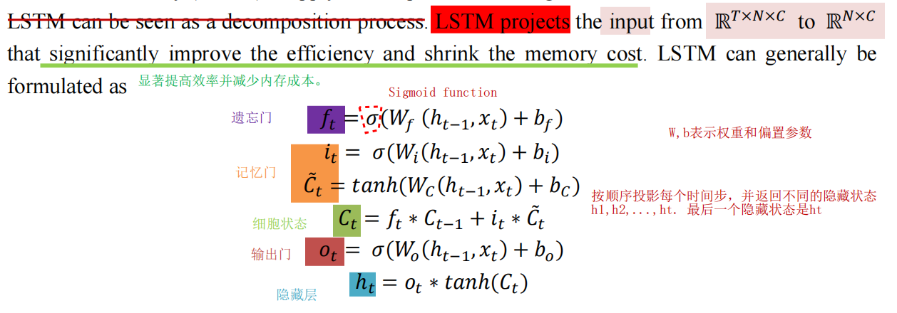

4 Experiments and Results

In this section , We conducted experiments on three real road networks , To answer :(1) Compared with the most advanced method at present , Whether the proposed traffic transformer model will significantly improve the prediction performance ?(2) Traffic Transformer Whether the model will extract features dynamically and hierarchically through the attention mechanism ?(3) Whether potential spatial global and local relationships will be extracted ? All the experiments were conducted in NVIDIA RTX 2080Ti GPU (11GB RAM) On the computing platform . Use Python To conduct and evaluate all experiments .

4.1 Data description

Our model is validated on three traffic data sets . One of them (METR-LA) Is the public data set published by the previous work , the other one (Urban-BJ, Ring-BJ) We made it ourselves .

say concretely ,METR-LA It was collected by loop detectors on the Los Angeles County highway . The data set range is 2012 year 3 Month to 2012 year 6 month , share 207 A sensor ( node ).UrbanBJ and Ring-BJ Is uploaded by Beijing 10000 More than one taxi GPS Data generated .Urban-BJ and Ring-BJ Of The time frame is 2015 year 6 Month to 2015 year 8 month . stay Urban-BJ in , Select a downtown area 278 Nodes .Ring-BJ The second ring road in Beijing is selected 236 Nodes . These nodes and road networks are as follows chart 4 Shown . Such as surface 1 Shown ,METR-LA Only the highway ,Ring-BJ Only class I highways are included . But the city of Beijing consists of different levels of roads .METR-LA Large area , Ring - bj In the middle ,Urban-BJ On a small scale . City - Beijing is a small city with mixed roads of different grades , It is a complex road network . The network around Beijing is very simple , It includes only one loop .METR-LA The complexity of is in the middle . We selected these data sets with different characteristics to test Traffic Transformer Performance in different situations .

4.2 Measures of effectiveness

In this study , We use three effectiveness measures , Mean absolute error (MAE)、 Mean absolute percentage error (MAPE) And root mean square error (RMSE), To evaluate the accuracy of the prediction model :

Among these different effectiveness measures ,MAE It measures the overall accuracy ;MAPE It is particularly sensitive to the error of low-speed mode , And measure whether the model tracks the congestion in the road network ;RMSE It measures the deviation and variance of the uncertainty of the forecast .

4.3 Model comparisons

What we proposed Traffic Transformer The model is similar to the following 5 Three benchmark models are compared , These include ARIMA and FC-LSTM Wait for the traditional model , as well as DCRNN、STGCN and GWN Based on gcn Model of .
*ARIMA: Common models in time series prediction . Autoregressive order 、 The difference and moving average are ARIMA Three key parameters of the model . adopt “auto-ARIMA” The tool performs grid search to obtain the optimal parameters .

• FC-LSTM: Complete connection LSTM (fully connected LSTM, FC-LSTM) It can extract the long-term and short-term dependencies of time features , It's a classic RNN, Learning time series by fully connected neural network and forecasting .
• DCRNN: Diffusion convolution recurrent neural network (Diffusion Convolutional Recurrent Neural Network, DCRNN) It is the most representative traffic forecast GNN One method . This paper presents a new method with encoder - Sequence to sequence of decoder structure (seq2seq) Model , For multi-step prediction .
• STGCN: Spatiotemporal graph convolution network (spatial - temporal Graph Convolutional Network, STGCN) It is another of the most representative traffic forecasts GNN Method . It uses the superposition of time blocks and space blocks , extract st - Feature and make one-step prediction .
• GWN: Graph Wave Net (GWN) take Wave Net Model applied to graph problem , Achieved the most advanced performance .

Besides , For further proof Traffic Transformer Effectiveness of different parts , We designed an ablation study , Three variants are used to match Traffic Transformer Compare :

• Traffic Transformer Encoder: Only the global encoder is used in the transformer structure , Completely cancel the global local decoder . therefore , The model does not need to define the neighborhood matrix in advance . The graph structure is completely obtained through model learning .
• Traffic Transformer Decoder: Only the global local decoder is used in the transformer structure , The global encoder is completely removed . Due to lack of global encoder , Therefore, the second multi header attention layer of the global local decoder is not established , And delete it . therefore , This model can also be regarded as a global encoder with mask .
• Traffic Transformer-No temporal: Remove the time embedding at the beginning of the model . This model can not extract the temporal characteristics of data . The velocity of different time steps is flattened on one dimension by linear neural network , Project onto the original dimension .

The grid search For tuning super parameters . Last , We set up Global Encoder Block and Global- local Decoder The number of blocks is 6. We embed time into the model after Hidden feature channels set to 64.Traffic Transformer Of feedforward network The dimension is set to 256. Let's minimize MAE To train our models , And use Adam As 1e-5 Optimizer for weight attenuation . An early stop on the validation set is used to mitigate over fitting . The shear gradient mechanism is used to stabilize the gradient , Improve the training effect .

surface 1 To table 3 Listed separately METR-LA、Urban BJ and Ring BJ The results of different traffic transformers and comparison benchmark methods . It turns out that ,TrafficTransformer and Traffic Transformer Encoder It has the best performance on three datasets and different predictors ( but GWN In the ring - BJ On the short term (15min) And the middle (30min) RMSE Is better ), Especially in the long run (60min) Forecasting , because Traffic Transformer Can benefit from extracting hidden long-distance spatial relationships . Through further analysis , Some observations and phenomena can be obtained .

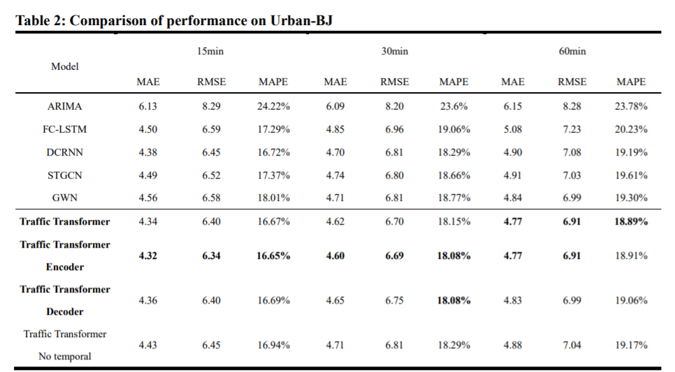
• In the results of the traditional model ,FC-LSTM Than ARIMA It's much better , This shows that the deep learning method is more suitable for traffic prediction .
• be based on gcn The model has higher accuracy than the traditional model . These are based on gcn The model shows that spatial features play an irreplaceable role in traffic forecasting . let me put it another way , The performance of spatiotemporal model is much better than that of temporal model .
• GWN、Traffic Transformer and Traffic Transformer Encoder Than DCRNN and STGCN Better results , because GWN Each iteration can learn an adaptive adjacency matrix ,Traffic Transformer and Traffic Transformer Encoder The adjacency relationship of each pair of nodes can be given through the attention mechanism . therefore ,GWN、 Traffic transformer and traffic transformer encoder can extract hidden spatial features , Especially in the long-term performance .
• And GWN comparison , In traffic transformer and traffic transformer encoder , The learned spatial relationships come from the multi headed attention mechanism , Therefore, the learned spatial relationship is dynamic , Rely on input data . The deep structure of traffic transformer and traffic transformer encoder extracts hierarchical spatiotemporal features , Instead of a single adjacent matrix . therefore , Our model dynamically extracts hierarchical hidden spatial features in different situations , Better than in long-term prediction GWN.
• stay Urban-BJ in , Ablation model Traffic Transformer Encoder Better than the original model , The best results have been achieved . This is because poorly defined neighborhood matrix will damage the model .Urban-BJ The complexity of is shown in the table 1 Shown , It is difficult to define a good enough adjacency matrix . therefore , For similar situations , It's best to use only Traffic Transformer Encoder instead of Traffic Transformer.
• Even if there is no time to embed blocks ,Traffic Transformer The result is not bad . It is simple to explain the time characteristics hidden in the data , No need to repeatedly extract the change of time dimension . At the beginning , Only a single time embedding is enough , And it can significantly reduce the training cost of decomposition .

We are still in the largest data set Urban BJ Compared with Traffic Transformer And DCRNN、STGCN and GWN Calculated cost of . Such as surface 3 Shown , because DCRNN The training cost of multi-step prediction architecture is too high , therefore DCRNN Is much slower than other models . our Traffic Transformer Compare... In training DCRNN fast , But more than STGCN and GWN slow . In the test , The efficiency of the one-step prediction model is remarkable ,Traffic Transformer Than DCRNN fast , But more than STGCN and GWN slow .

4.4 Model Interpretation

Our experiments show that , The model with learnable adjacency matrix can better learn spatial relations , Especially in terms of long-term forecasting . In the global encoder and the global local decoder , The traffic converter learns spatial relationships through multiple heads of attention . The dynamics of each bull's attention 、 The hierarchical attention matrix is similar to the adjacent matrix , It can reveal the learned spatial relationship .

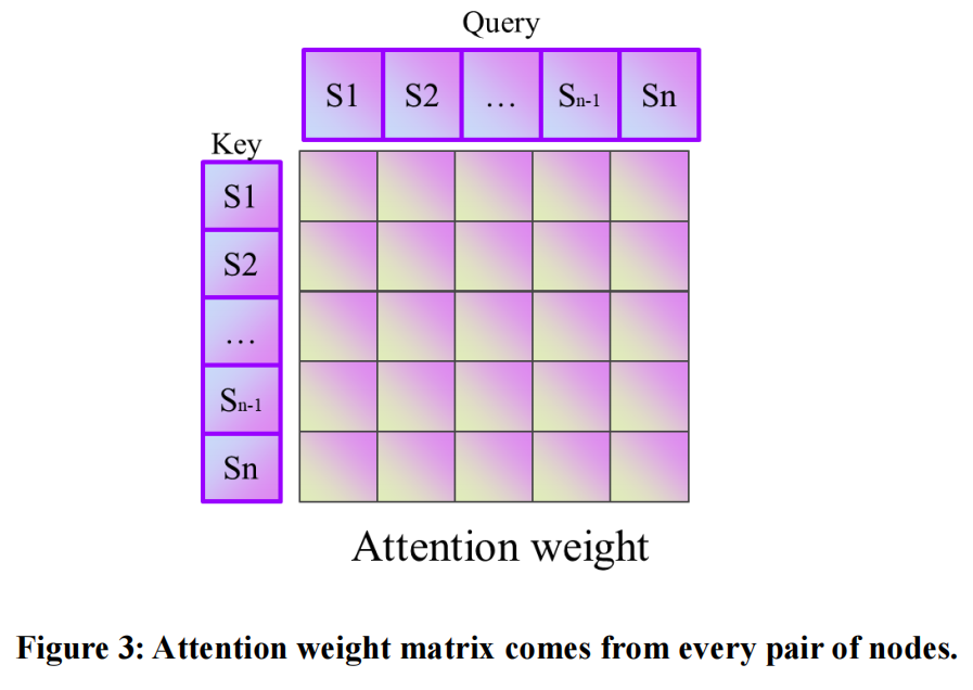
We designed another experiment , To better show Traffic Transformer The dynamic and hierarchical spatiotemporal characteristics of learning . Select several batches of test data and project them into the training model , Return to the attention weight matrix for analysis . for example , We are metro - la Three batches were selected in the test set of , Respectively in 0:00 AM、8:00AM、4:00PM Three different time periods . These batches are projected into our trained models . The attention weight matrix of each multi head attention layer and each data set is scaled to (0,1), Such as chart 5 Shown .Global The attention weight matrix in the encoder is called “ Source right ”, In the figure, it is abbreviated as “src”;Global- local The first attention weight matrix in the decoder is called “ Target right ”, In the figure, it is abbreviated as “tgt”;Global- local The second attention weight matrix in the decoder is called “ Memory rights ”, In the figure, it is abbreviated as “mem”.

chart 5： Attention weight matrix in different time periods .（a） ： Notice the weight matrix 0:00 AM batch ;（b） ： Pay attention to the morning 8:00 Weight matrix of the batch ;（c） Pay attention to the afternoon 4:00 Weight matrix of the batch .

In the heat map of each focus weight , The second of weight $i$ Xing He $j$ Column means $senso{r}_i$ and $senso{r}_j$ Influence . Such as chart 5 Shown , Some rows and columns have much larger weights than others , This means that the nodes corresponding to these rows and columns are important to almost all other nodes . This shows that , These nodes affect most of the nodes in the graph , The impact of other nodes is weak . Different periods 、 Different levels of source concern have different weights ,Traffic Transformer It can dynamically extract global spatial features based on input data . The goal attention weights look very similar . This is because the target attention weight uses a predefined K-hop Adjacency matrix to focus on local . Memory attention weights indicate how global and local features are fused . Their graphs show features similar to the source concern weight Heatmap , Some nodes in the fusion graph affect most nodes , Others don't .

To further substantiate our observations , We define The importance of each node


among , Nodes whose mean value is greater than one standard deviation are defined as Impact nodes .

1) Dynamicity

We are metro - la Two batches of data were selected in the test set . One in the morning 8 spot , The other is in the afternoon 4 spot . Send these two batches of data to the trained model , And return the attention weight matrix in all multi head attention blocks together with the output . We choose “ memory 6” Attention weight matrix ( namely : For further analysis . choice 144 No. 1 sensor for analysis . selection 144 The most influential of the No. 1 sensors 10 A sensor , Draw on chart 6 in . Pictured 6 Shown , Red dot means NO.144 sensor . The blue dot indicates the morning 8:00 The time period has the greatest impact 10 A sensor , Orange dots indicate afternoon 4:00 The time period has the greatest impact 10 A sensor . The blue dot is in the east of the network , The red dot is located in the west of the network . It's important to point out that ,162 Sensor No. 1 and 163 Sensor No. 1 is very close , But as shown in the picture 6 The enlarged part shows , They are located in different directions of the same highway section . It means Traffic Transformer Different influence points have been found in different time periods . It shows us that Traffic Transformer Spatial dependencies can be extracted dynamically , Adjacency is dynamic in our model , Dependent on input . It breaks through the traditional gcn The fixed limit of adjacent matrix in the model of , Better performance .

Fig.6 144 The influence of sensor No. 1 in different time periods . Blue dot : In the morning 8:00; Orange dots : Afternoon 4 spot . The enlarged picture shows two sensors in different directions on the same road .

2) Hierarchy

stay metro - la Data set , We selected in the test set 8:00AM A batch of data . We calculate the influence nodes of different source attention layers , And draw it on a map , Pictured 7 Shown . It can be seen that , Most of the affected nodes are located near the usually important intersections in the traffic network . The spatial features of different levels show the hierarchical features from global to local and then to global . At the bottom ( chart 7 (a), The first 1 layer ), The affected nodes are distributed throughout the network . But in the middle ( chart 7 (b) and , The first 2 Tier and tier 4 layer ), The affected nodes are concentrated in a part of the network . for example , chart 7 (b) The cyan dots representing the second layer of influence nodes are mostly concentrated in the east of the network . At higher levels ( chart 7 (d), The first 6 layer ), The affected nodes are distributed in the whole network again . It's important to point out that , Interestingly , In the 6 The sensor is extracted from the layer 26( Left side of the picture ) As the influence node . However , stay metro - la in , The first 26 A point is an isolated vertex . prove Traffic Transformer Can extract long-distance spatial features .

Fig.7 chart 7: Influence nodes of different layers on the map :(a) The first 1 layer ;(b) 2 layer ;(c) The fourth level ;(d) layer 6.(a) For the underlying ;(b) and (c) It's the middle layer ;(d) It's the top floor .(a) and (d) Prefer global features ,(b) and (c) Prefer local features .

5 Conclusions and Discussions

In this paper , We propose a new spatio-temporal map modeling and long-term traffic forecasting model . The traffic transformer model proposed by us can 、 Effectively extract dynamics from data 、 Layered traffic space-time characteristics . We select three different data sets to evaluate whether our model is robust in different situations . Compare this model with the traditional model 、 be based on gcn Model and ablation model, etc 8 Three benchmark models are compared . Three effectiveness measures (MAE, MAPE and RMSE) Used to evaluate the accuracy of these models . On three real datasets ,Traffic Transformer The most advanced results have been achieved . Help people find hierarchical nodes in the network .

According to the experimental results , We can draw the following conclusion :(a) Network wide traffic prediction has similar characteristics and challenges to naturallanguageprocessing . Transformer and other advanced naturallanguageprocessing methods and frameworks can adapt to the whole network traffic prediction problem .(b) In all traffic forecasting models ,traffic Transformer The best prediction results were obtained within the acceptable training time . This proves Transformer Powerful function in traffic forecasting problem . After training Traffic Transformer The influential sensors for model extraction are not local . This indicates that the spatial dependence of road network may vary greatly in distance , The traditional distance based adjacency matrix has some limitations .(d) Different time periods have different influence sensors , It means that the spatial dependency of road network is dynamic , The traditional fixed adjacency matrix has limitations .(d) Spatial dependencies are hierarchical , Depth models can extract these features globally or locally .（e） With the increase of network complexity , It is more and more difficult to define a good enough adjacency matrix , And the harm of the artificial definition of matrix to the model is more and more inevitable . Let the model learn spatial correlation to better improve performance in these cases . However , When the network complexity is moderate , Use a predefined neighborhood matrix to help the model better understand “ Local ” Can improve performance .

In the future work , The model can be extended to more external information ( Such as road features 、 Adverse weather conditions and major events ), To improve the prediction accuracy . Due to the limitation of data , This paper only studies speed prediction in road network , But once there is more information data , The model can be extended to other traffic states ( Such as flow and density ) And other transportation systems ( Such as subway network and non motor vehicle transportation system ). This paper limits the number of sensors to 300 Below . This is because Transformer Yes $O(n^2)$ When the number of sensors is too large , The model will be difficult to train . However , Recently proposed Transformer Some variations of , Such as Transformer- xl (Dai etc. . and Longformer (Beltagy etc. ., 2020 year ) It can handle long documents and other ten thousand level sequences . We will study the use of Transformer To handle larger networks , And find deeper hidden dependencies in the traffic . Besides , be based on Transformer The language model of is in NLP It's also popular in , Such as BERT (Devlin et.al 2018) and GPT (Radford et.al)., 2017; Redford press ., 2018). The researchers believe that BERT It is an automatic encoding (AE) The process , and GPT It's an autoregression (AR) The process . In the extraction of traffic spatiotemporal features , The spatial dimension is more like a AE The process , The time dimension is more like a AR The process . In future research , One “ Language model ” Of traffic may show great performance .

---