当前位置:网站首页>Numerical calculation method chapter7 Calculating eigenvalues and eigenvectors of matrices
Numerical calculation method chapter7 Calculating eigenvalues and eigenvectors of matrices
2022-06-23 06:40:00 【Espresso Macchiato】
0. Problem description
The problem in this chapter is to say , Given a n n n Order matrix , How to solve its eigenvalue numerically , namely :
A x = λ x Ax = \lambda x Ax=λx
1. Power law
1. Ideas
In fact, the main idea of power method still comes from the idea of iteration .
obviously , For any vector x ⃗ \vec{x} x, We can always use it n n n A set of orthogonal bases of order matrix , namely :
x ⃗ = ∑ i = 1 n x i ⋅ n i ⃗ \vec{x} = \sum_{i=1}^{n} x_i \cdot \vec{n_i} x=i=1∑nxi⋅ni
among , n i ⃗ \vec{n_i} ni For matrix A A A A unit vector of , Yes A n i ⃗ = λ i n i ⃗ A\vec{n_i} = \lambda_i \vec{n_i} Ani=λini.
Make x ⃗ ( 0 ) = ∑ i x i n i ⃗ \vec{x}^{(0)} = \sum_{i}x_i \vec{n_i} x(0)=∑ixini, x ⃗ ( k + 1 ) = A x ⃗ ( k ) \vec{x}^{(k+1)} = A\vec{x}^{(k)} x(k+1)=Ax(k), Easy to have :
x ⃗ ( k ) = ∑ i x i ⋅ λ i k ⋅ n i ⃗ \vec{x}^{(k)} = \sum_{i} x_i \cdot \lambda_i^k \cdot \vec{n_i} x(k)=i∑xi⋅λik⋅ni
The corresponding module length is :
∣ ∣ x ⃗ ( k ) ∣ ∣ = ∑ i x i 2 λ i 2 k ||\vec{x}^{(k)}|| = \sqrt{\sum_i x_i^2 \lambda_i^{2k}} ∣∣x(k)∣∣=i∑xi2λi2k
Let's consider being k → ∞ k \to \infty k→∞ when x ⃗ ( k ) \vec{x}^{(k)} x(k) The direction of , Might as well set m a x ( ∣ λ i ∣ ) = λ max(|\lambda_i|) = \lambda max(∣λi∣)=λ.
Might as well set λ = ∣ λ 1 ∣ ≥ ∣ λ 2 ∣ ≥ . . . ≥ ∣ λ n ∣ \lambda = |\lambda_1| \geq |\lambda_2| \geq ... \geq |\lambda_n| λ=∣λ1∣≥∣λ2∣≥...≥∣λn∣, Then we can discuss according to the situation :
Suppose there is only one positive λ i \lambda_i λi bring ∣ λ i ∣ = λ |\lambda_i| = \lambda ∣λi∣=λ
lim k → ∞ x ⃗ ( k ) ∣ ∣ x ⃗ ( k ) ∣ ∣ = n 1 ⃗ \lim_{k \to \infty} \frac{\vec{x}^{(k)}}{||\vec{x}^{(k)}||} = \vec{n_1} k→∞lim∣∣x(k)∣∣x(k)=n1
At this time there is :
x ⃗ ( k + 1 ) = A x ⃗ ( k ) = λ x ⃗ ( k ) \vec{x}^{(k+1)} = A\vec{x}^{(k)} = \lambda \vec{x}^{(k)} x(k+1)=Ax(k)=λx(k)
Assume that ∣ λ i ∣ = λ |\lambda_i| = \lambda ∣λi∣=λ Conditions of the i i i share m m m individual , And there are λ i > 0 \lambda_i > 0 λi>0
lim k → ∞ x ⃗ ( k ) ∣ ∣ x ⃗ ( k ) ∣ ∣ = ∑ i m x i ∑ i m x i 2 n i ⃗ \lim_{k \to \infty} \frac{\vec{x}^{(k)}}{||\vec{x}^{(k)}||} = \sum_{i}^{m}\frac{x_i}{\sqrt{\sum_i^m x_i^2}}\vec{n_i} k→∞lim∣∣x(k)∣∣x(k)=i∑m∑imxi2xini
There are also :
x ⃗ ( k + 1 ) = A x ⃗ ( k ) = λ x ⃗ ( k ) \vec{x}^{(k+1)} = A\vec{x}^{(k)} = \lambda \vec{x}^{(k)} x(k+1)=Ax(k)=λx(k)
Suppose there is m m m A positive ∣ λ i ∣ = λ |\lambda_i| = \lambda ∣λi∣=λ, l l l A negative ∣ λ i ∣ = λ |\lambda_i| = \lambda ∣λi∣=λ
lim k → ∞ x ⃗ ( k ) ∣ ∣ x ⃗ ( k ) ∣ ∣ = ∑ i m x i ∑ i m + l x i 2 n i ⃗ + ∑ j l ( − 1 ) k ⋅ x j ∑ i m + l x j 2 n j ⃗ \lim_{k \to \infty} \frac{\vec{x}^{(k)}}{||\vec{x}^{(k)}||} = \sum_{i}^{m}\frac{x_i}{\sqrt{\sum_i^{m+l} x_i^2}}\vec{n_i} + \sum_{j}^{l}\frac{(-1)^{k} \cdot x_j}{\sqrt{\sum_i^{m+l} x_j^2}}\vec{n_j} k→∞lim∣∣x(k)∣∣x(k)=i∑m∑im+lxi2xini+j∑l∑im+lxj2(−1)k⋅xjnj
here , although x ⃗ ( k + 1 ) / x ⃗ ( k ) \vec{x}^{(k+1)} / \vec{x}^{(k)} x(k+1)/x(k) unstable , But there is still :
x ⃗ ( k + 2 ) = A A x ⃗ ( k ) = λ 2 x ⃗ ( k ) \vec{x}^{(k+2)} = AA\vec{x}^{(k)} = \lambda^2 \vec{x}^{(k)} x(k+2)=AAx(k)=λ2x(k)
But here's the thing , What is discussed here is only a general case , It is based on the assumption that all x i ≠ 0 x_i \neq 0 xi=0, If the projection on some components happens to be 0, That is, some x i = 0 x_i = 0 xi=0, Then the above discussion will change or even fail .
and , As analyzed above , By the power method , We can only obtain the eigenvalue with the largest absolute value in a general matrix λ \lambda λ, Unable to get all its characteristic values , This also needs attention .
2. Canonical operation
Based on the above ideas , We give the normal operation method of power method :
{ y ⃗ ( k ) = x ⃗ ( k ) / ∣ ∣ x ⃗ ( k ) ∣ ∣ x ⃗ ( k + 1 ) = A ⋅ y ⃗ ( k ) \left\{ \begin{aligned} \vec{y}^{(k)} &= \vec{x}^{(k)} / ||\vec{x}^{(k)}|| \\ \vec{x}^{(k+1)} &= A \cdot \vec{y}^{(k)} \end{aligned} \right. { y(k)x(k+1)=x(k)/∣∣x(k)∣∣=A⋅y(k)
Through the above iteration , We can find the matrix A A A The absolute value of the maximum eigenvalue .
3. Pseudo code implementation
give python The pseudo code is implemented as follows :
def power_fn(A, epsilon=1e-6):
    n = len(A)
    x = [1 for _ in range(n)]
    for _ in range(10**3):
        s = math.sqrt(sum(t*t for t in x))
        y = [t/s for t in x]
        z = [0 for _ in range(n)]
        for i in range(n):
            for j in range(n):
                z[i] += A[i][j] * y[j]

        lamda = sum([a/b for a, b in zip(z, y)]) / n
        delta =  max(abs(a-b) for a, b in zip(z, x))
        x = z
        if delta < epsilon:
            break
    return lamda
Of course , Only the maximum absolute value with a single sign is considered here λ \lambda λ The situation of , If there is a maximum eigenvalue with the same absolute value and the opposite sign λ \lambda λ, The above code will fail , Some complex operations and judgments are required , This is just a lot of expansion .
2. Inverse power method
1. Ideas & Method
The idea of inverse power method is not different from that of power method , But the power method iterates directly forward , namely :
x ⃗ ( k + 1 ) = A x ⃗ ( k ) \vec{x}^{(k+1)} = A \vec{x}^{(k)} x(k+1)=Ax(k)
The iteration method of the inverse power method is :
x ⃗ ( k + 1 ) = A − 1 x ⃗ ( k ) \vec{x}^{(k+1)} = A^{-1} \vec{x}^{(k)} x(k+1)=A−1x(k)
Or say :
x ⃗ ( k ) = A x ⃗ ( k + 1 ) \vec{x}^{(k)} = A \vec{x}^{(k+1)} x(k)=Ax(k+1)
For the solution , We only need to add the method of solving multivariate equations in the previous chapter on the basis of the above power method .
What needs to be added is , Because the iteration used here is the opposite of the power method , therefore , The solution here is A − 1 A^{-1} A−1 The eigenvalue with the largest absolute value , That is to say A A A The eigenvalue with the smallest absolute value .
And the same , The additional implicit condition here is the need for a matrix A A A It's full rank , Otherwise, there is no inverse matrix , The above equation x ⃗ ( k ) = A x ⃗ ( k + 1 ) \vec{x}^{(k)} = A \vec{x}^{(k+1)} x(k)=Ax(k+1) There may be no solution .
2. Pseudo code implementation
alike , Here we give the simplest case ( namely A A A The case of full rank and only one minimum absolute eigenvalue ), Of the inverse power method python Pseudo code implementation :
def rev_power_fn(A, epsilon=1e-6):
    n = len(A)
    x = [1 for _ in range(n)]
    for _ in range(10**3):
        s = math.sqrt(sum(t*t for t in x))
        y = [t/s for t in x]
        z = loose_iter(A, y)

        lamda = sum([a/b for a, b in zip(y, z)]) / n
        delta =  max(abs(a-b) for a, b in zip(z, x))
        x = z
        if delta < epsilon:
            break
    return lamda
3. Of a real symmetric matrix Jacobi Method
1. Ideas & Method
As mentioned earlier , Power method and anti power method are essentially to find a stable eigenvector through the idea of iteration , Then the eigenvalue is calculated by eigenvector .
therefore , They can only find an eigenvalue of the matrix , It is impossible to solve all eigenvalues of a matrix . If you want to solve all the eigenvalues of the matrix , The above methods will fail .
however , For some special matrices , That is, a real symmetric matrix , In fact, we can solve all the eigenvalues , A typical method is Jacobi Method .
In essence ,Jacobi The method still iterates , However, the idea of iteration is to continuously carry out unitary transformation on the matrix , Make it converge to a diagonal matrix , In this case, each diagonal element of the diagonal matrix is the eigenvalue of the original matrix .
To be specific , It is known that A x = λ x Ax = \lambda x Ax=λx, There are orthogonal matrices U U U Satisfy U U T = I UU^{T} = I UUT=I, Then there are :
U A U T ⋅ U x = λ ⋅ U x UAU^{T} \cdot Ux = \lambda \cdot Ux UAUT⋅Ux=λ⋅Ux
here , λ \lambda λ Still matrix U A U T UAU^{T} UAUT The eigenvalues of the .
If after a series of transformations :
U k U k − 1 . . . U 1 A U 1 T U 2 T . . . U k T = d i a g ( λ 1 , . . . , λ n ) U_kU_{k-1}...U_{1}AU_1^{T}U_2^{T}...U_{k}^T = diag(\lambda_1, ..., \lambda_n) UkUk−1...U1AU1TU2T...UkT=diag(λ1,...,λn)
be λ 1 , . . . , λ n \lambda_1, ..., \lambda_n λ1,...,λn That's the matrix A A A All eigenvalues of .
The remaining question is how to solve these matrices U U U,Jacobi A feasible idea given by the method is Givens matrix , namely :
G ( p , q , θ ) = ( 1 . . . c o s θ . . . s i n θ . . . . . . − s i n θ . . . c o s θ . . . 1 ) G(p, q, \theta) = \begin{pmatrix} 1 \\ & ... \\ & & cos\theta & ... & sin\theta \\ & & ... & & ... \\ & & -sin\theta & ... & cos\theta \\ & & & & & ... \\ & & & & & & 1 \end{pmatrix} G(p,q,θ)=⎝⎜⎜⎜⎜⎜⎜⎜⎜⎛1...cosθ...−sinθ......sinθ...cosθ...1⎠⎟⎟⎟⎟⎟⎟⎟⎟⎞
in other words , Only right p , q p,q p,q The elements of the two lines proceed at an angle of θ \theta θ The rotation transformation of .
Make :
B = G ( p , q , θ ) ⋅ A ⋅ G T ( p , q , θ ) B = G(p,q,\theta) \cdot A \cdot G^{T}(p,q,\theta) B=G(p,q,θ)⋅A⋅GT(p,q,θ)
Then there are :
{ b i , j = a i , j b i , p = b p , i = a p , i c o s θ − a q , i s i n θ b i , q = b q , i = a p , i s i n θ + a q , i c o s θ b p , p = a p , p c o s 2 θ + a q , q s i n 2 θ − a p , q s i n 2 θ b q , q = a p , p s i n 2 θ + a q , q c o s 2 θ + a p , q s i n 2 θ b p , q = b q , p = a p , q c o s 2 θ + a p , p − a q , q 2 s i n 2 θ \left\{ \begin{aligned} b_{i, j} &= a_{i, j} \\ b_{i,p} &= b_{p,i} = a_{p, i}cos\theta - a_{q, i}sin\theta \\ b_{i,q} &= b_{q,i} = a_{p, i}sin\theta + a_{q, i}cos\theta \\ b_{p,p} &= a_{p,p}cos^{2}\theta + a_{q,q}sin^{2}\theta - a_{p,q}sin2\theta \\ b_{q,q} &= a_{p,p}sin^{2}\theta + a_{q,q}cos^{2}\theta + a_{p,q}sin2\theta \\ b_{p,q} &= b_{q,p} = a_{p,q} cos2\theta + \frac{a_{p,p} - a_{q,q}}{2}sin2\theta \end{aligned} \right. ⎩⎪⎪⎪⎪⎪⎪⎪⎪⎪⎪⎨⎪⎪⎪⎪⎪⎪⎪⎪⎪⎪⎧bi,jbi,pbi,qbp,pbq,qbp,q=ai,j=bp,i=ap,icosθ−aq,isinθ=bq,i=ap,isinθ+aq,icosθ=ap,pcos2θ+aq,qsin2θ−ap,qsin2θ=ap,psin2θ+aq,qcos2θ+ap,qsin2θ=bq,p=ap,qcos2θ+2ap,p−aq,qsin2θ
Let's take the right one θ \theta θ, bring b q , p = 0 b_{q,p} = 0 bq,p=0, Then there are :
{ ∑ i ≠ j b i , j 2 = ∑ i ≠ j a i , j 2 − 2 a p , q 2 ∑ i b i , i 2 = ∑ i a i , i 2 + 2 a p , q 2 \left\{ \begin{aligned} \sum_{i\neq j} b_{i,j}^2 &= \sum_{i\neq j} a_{i,j}^2 - 2a_{p,q}^2 \\ \sum_{i} b_{i,i}^2 &= \sum_{i} a_{i,i}^2 + 2a_{p,q}^2 \end{aligned} \right. ⎩⎪⎪⎪⎨⎪⎪⎪⎧i=j∑bi,j2i∑bi,i2=i=j∑ai,j2−2ap,q2=i∑ai,i2+2ap,q2
You can see , The absolute values of the elements of the off diagonal elements will become smaller and smaller .
therefore , After enough iterations , The original matrix can be A A A Transform into a near diagonal matrix with the same eigenvalue .
In order to further improve the speed of iteration , The off diagonal element with the largest absolute value can be selected first for iterative elimination .
2. Pseudo code implementation
alike , We give python The pseudo code is implemented as follows :
def jacobi_eigen_fn(A, epsilon=1e-6):
    n = len(A)
    assert(len(A[0]) == n)
    assert(A[i][j] == A[j][i] for i in range(n) for j in range(i+1, n))

    finished = False
    for _ in range(1000):
        for p in range(n):
            for q in range(p+1, n):
                if A[p][p] != A[q][q]:
                    theta = 0.5 * math.atan(2*A[p][q] / (A[q][q] - A[p][p]))
                else:
                    theta = math.pi / 4
                ap = deepcopy(A[p])
                aq = deepcopy(A[q])
                for i in range(n):
                    if i == p or i == q:
                        continue
                    A[i][p] = A[p][i] = ap[i] * math.cos(theta) - aq[i] * math.sin(theta)
                    A[i][q] = A[q][i] = ap[i] * math.sin(theta) + aq[i] * math.cos(theta)
                A[p][p] = ap[p] * math.cos(theta)**2 + aq[q] * math.sin(theta)**2 - ap[q] * math.sin(2*theta)
                A[q][q] = ap[p] * math.sin(theta)**2 + aq[q] * math.cos(theta)**2 + ap[q] * math.sin(2*theta)
                A[p][q] = A[q][p] = ap[q] * math.cos(2 * theta) + (ap[p] - aq[q])/2 * math.sin(2*theta)

                finished = all(A[i][j] < epsilon for i in range(n) for j in range(i+1, n))
                if finished:
                    break
            if finished:
                break
        if finished:
            break
    return [A[i][i] for i in range(n)]
边栏推荐
- 百度URL参数之LINK?URL参数加密解密研究(代码实例)
- haas506 2.0开发教程-sntp(仅支持2.2以上版本)
- Laravel log channel 分组配置
- Gridsearchcv (grid search), a model parameter adjuster in sklearn
- English语法_副词 - ever / once
- 什么是客户体验自动化?
- Machine learning artifact scikit learn minimalist tutorial
- Leetcode topic resolution single number II
- 微信小程序 - 全局监听globalData的某个属性变化,例如监听网络状态切换
- Day_ 08 smart health project - mobile terminal development - physical examination appointment
猜你喜欢

Easy EDA #学习笔记09# | ESP32-WROOM-32E模组ESP32-DevKitC-V4开发板 一键下载电路

中台库存中的实仓与虚仓的业务逻辑设计

Detailed explanation of redis persistence, master-slave and sentry architecture

C# wpf 通过绑定实现控件动态加载

Home address exchange

haas506 2.0開發教程-高級組件庫-modem.sms(僅支持2.2以上版本)
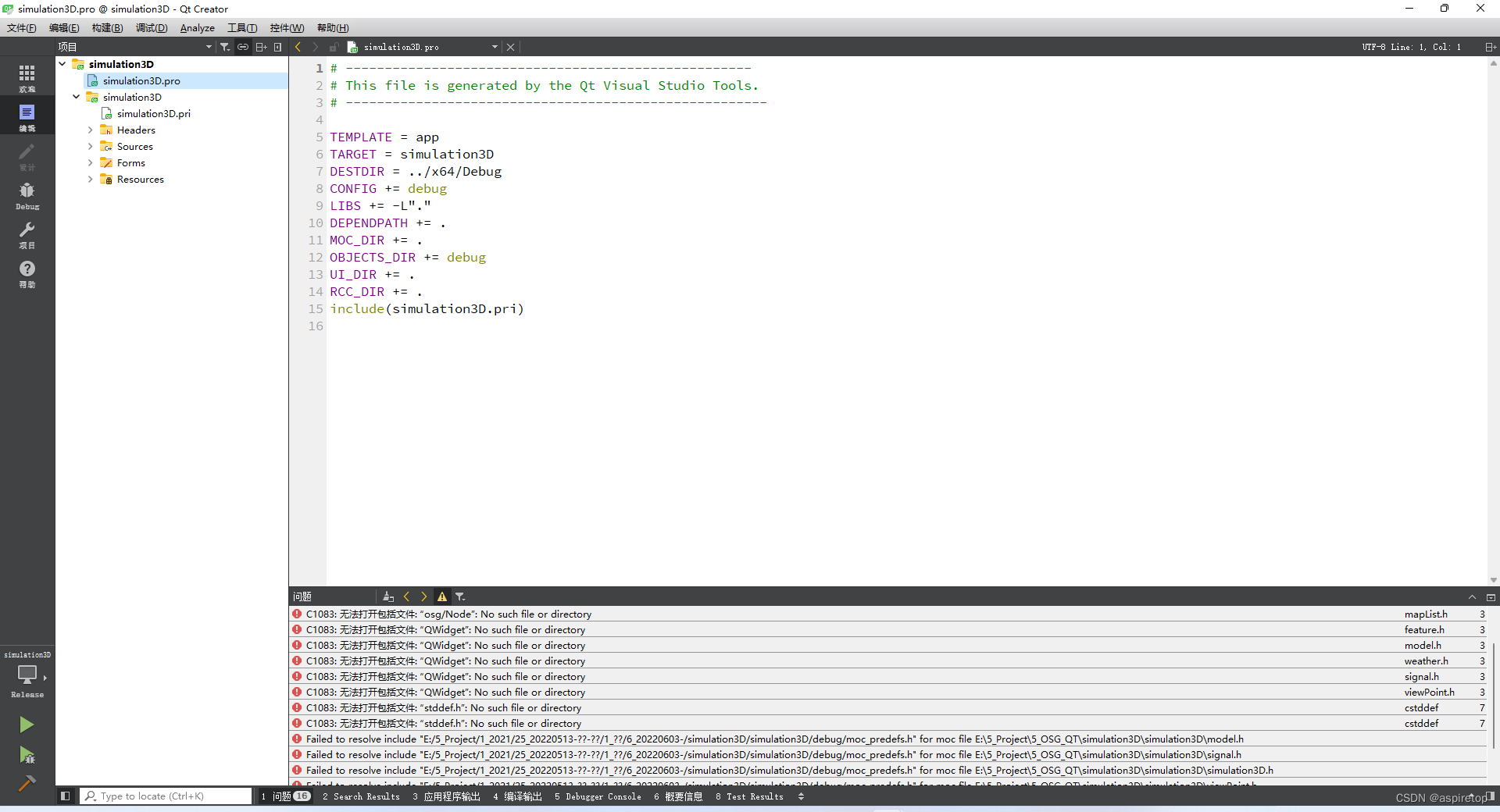
Vs+qt project transferred to QT Creator
百度URL参数之LINK?URL参数加密解密研究(代码实例)

QT creator builds osgearth environment (osgqt msvc2017)
vs+qt项目转qt creator

随机推荐
把CSMA/CD、Token Bus、Token Ring说清楚
杂七杂八的东东
Day_ 01 smart communication health project - project overview and environmental construction
坐标 转化
Leetcode topic resolution valid anagram
图解 Google V8 # 17:消息队列:V8是怎么实现回调函数的?
Repeated DNA sequences for leetcode topic resolution
haas506 2.0开发教程-hota(仅支持2.2以上版本)
解析创客教育中的造物原理
Illustration Google V8 18: asynchronous programming (I): how does V8 implement micro tasks?
Softing dataFEED OPC Suite将西门子PLC数据存储到Oracle数据库中
Illuminate\support\collection de duplication unique list de duplication
js创建数组(元素都是对象)
Coordinate transformation
Plot+seaborn+folium: a visual exploration of Abbey's rental housing data
解析创客教育中的个性化学习进度
CPU的功能和基本结构
Measurement principle and thickness measurement mode of spectral confocal
Smart port: how to realize intelligent port supervision based on the national standard gb28181 protocol easygbs?
百度URL參數之LINK?URL參數加密解密研究(代碼實例)