【深度学习】手把手教你写“手写数字识别神经网络“，不使用任何框架，纯Numpy

前言

  一直以来笔者对机器学习都很感兴趣，但由于大学主修专业与机器学习无关，所以一直没有时间(拖延症)不用框架来完整的写一个神经网络。不过好在这个学期正好有一门主修选修课程，借此机会发表一下自己的学习成果。

  学习这篇文章的前提是你有一定的Python、线性代数、高数知识，并且对全连接神经网络有一定的了解，知道全连接神经其实就是一个可以通过调参逼近任何函数的非线性函数(我是这么理解的，当然我也同样认为存在许多它不可能精确描述的函数)，知道前向传播和反向传播过程。

  如果你对神经网络有一定了解，但是又没有仔细思考 过建议可以先看一下B站3Blue1Brown关于深度学习 Deep Learning的视频，学完这个视频你就能对全连接神经网络有较为深刻的认识。当然你可能还是没有办法写出一个完整的神经网络，因为不少人可能对反向传播过程中矩阵的求导不是很了解，导致不能推导出反向传播过程梯度的计算公式。

手写数字识别神经网络设计

  假设你已经看过视频,或者对已经此已经比较了解了，那么下面就可以开始设计了。

  这里为了方便讲解以及使得第一个程序清晰！！！，就不使用MINIST数据集了。这里使用我学习的教程提供的一个数据集，这个数据集合看起来像这样，文件内容就是手写数字的图片数据，相当于二值化图片。命名规则：图片中的数字_序号 --> label_seq.txt。接下来就用标签称呼图片所写数字的值。现在的重点不在于数据集，所以这里直接给出加载数据及的函数。点击这里下载数据集。

# 函数img2vector将图像转换为向量
from numpy import *
from os import listdir

def img2vector(filename):
    returnVect = np.zeros((1, 1024))
    fr = open(filename)
    for i in range(32):
        lineStr = fr.readline()
        for j in range(32):
            returnVect[0, 32 * i + j] = int(lineStr[j])
    return returnVect
    
# 读取手写字体txt数据
def handwritingData(dataPath):
    hwLabels = []
    FileList = listdir(dataPath)  # 1 获取目录内容
    m = len(FileList)
    np.Mat = np.zeros((m, 1024))
    for i in range(m):
        # 2 从文件名解析分类数字
        fileNameStr = FileList[i]
        fileStr = fileNameStr.split('.')[0]  # take off .txt
        classNumStr = int(fileStr.split('_')[0])
        hwLabels.append(classNumStr)
        np.Mat[i, :] = img2vector(dataPath + '/%s' % fileNameStr)
    return np.Mat, hwLabels

数据集使用

将数据集解压到指定目录下，like this:

..
└ Work Folder
	└ Net.py
	  trainingDigits
      testDigits

# 读取训练数据
trainDataPath = "./trainingDigits"
trainMat, trainLabels = handwritingData(trainDataPath)

trainMat.shape -> (1934, 1024)
trainMat[i]对应的标签为trainLabels[i]

神经网络设计

  这里是模型是这样的，如上图，一个输入层，两个隐含层，激活函数选择Sigmod,损失函数选择误差平方和函数（我这么称呼的，不知道叫什么），如下面所示。建议第一次自己些的话损失函数就用误差平方和函数，以为这个损失函数简单，求导方便，便于学习，后面可以在此基础上进行改进。

Cost ：代价，在这里也就是需要计算的Loss值。
$$\begin{gathered} Sigmod(x)=\frac{1}{1+e^{-x}} \\ Sigmo{d}^{\prime }(x)=Sigmod(x)(1-Sigmod(x)) \end{gathered}$$
$$误差平方和函数:Cost(\hat{y},y)=\frac{1}{2}(\hat{y}-y{)}^2$$

  如果数学能力不够强的话建议不要用像交叉熵损失函数，也不要用Softmax激活函数这些求导麻烦的函数，不利于学习。

数学模型

$符号：A^{(层)}$
$S=Sigmod$

---

$$维度：|{\mathbf{x}}_{1024x1}|{\mathbf{W}}_{16x1024}^{(1)}|{\mathbf{b}}_{16x1}^{(1)}|{\mathbf{W}}_{16x16}^{(2)}|{\mathbf{b}}_{16x1}^{(2)}|{\mathbf{W}}_{10x16}^{(3)}|{\mathbf{b}}_{10x1}^{(3)}|{\hat{\mathbf{y}}}_{10\mathbf{x}1}|$$

---

$前向传播：$
${\mathbf{z}}^{(l)}={\mathbf{W}}^{(l)}{\mathbf{a}}^{(l-1)}+{\mathbf{b}}^{(l)}$
${\mathbf{a}}^{(l)}=f\left({\mathbf{z}}^{(l)}\right)$
$\hat{\mathbf{y}}={\mathbf{a}}^{(L)}=f\left({\mathbf{z}}^{(L)}\right)$
$\mathcal{L}=\mathcal{L}(\mathbf{y},\hat{\mathbf{y}})$

$\mathbf{x}=a^{(0)}也就是输入的图片数据$
${\mathbf{z}}^{(1)}={\mathbf{W}}^{(1)}{\mathbf{a}}^{(0)}+{\mathbf{b}}^{(1)}$
${\mathbf{a}}^{(1)}=S({\mathbf{z}}^{(1)})$

${\mathbf{z}}^{(2)}={\mathbf{W}}^{(2)}{\mathbf{a}}^{(1)}+{\mathbf{b}}^{(2)}$
${\mathbf{a}}^{(2)}=S({\mathbf{z}}^{(2)})$

${\mathbf{z}}^{(3)}={\mathbf{W}}^{(2)}{\mathbf{a}}^{(2)}+{\mathbf{b}}^{(3)}$
$\hat{\mathbf{y}}=S({\mathbf{z}}^{(3)})预测结果，最大值下标就是预测的数字结果$

$Loss=Cost(\hat{\mathbf{y}},\mathbf{y})$

---

$反向传播:\odot 是对应元素相乘$

$\frac{\partial Loss}{\partial \hat{\mathbf{y}}}$:这里是对应元素求导

输出层：
$$\begin{gathered} {\mathbf{\delta }}^{(L)}={\nabla }_{{\mathbf{a}}^{(L)}}\mathcal{L}\odot S^{\prime }\left({\mathbf{z}}^{(L)}\right)=\frac{\partial Loss}{\partial \hat{\mathbf{y}}}\odot S^{\prime }\left({\mathbf{z}}^{(L)}\right)=\frac{\partial \mathcal{L}}{\partial {\mathbf{z}}^{(L)}} \\ 这里求得：\frac{\partial Loss}{\partial \hat{\mathbf{y}}}\odot S^{\prime }\left({\mathbf{z}}^{(3)}\right) \end{gathered}$$
其他层套用公式：
$$\begin{gathered} {\mathbf{\delta }}^{(l)}=\left({\left({\mathbf{W}}^{(l+1)}\right)}^{\mathrm{T}}{\mathbf{\delta }}^{(l+1)}\right)\odot S^{\prime }\left({\mathbf{z}}^{(l)}\right) \\ \frac{\partial \mathcal{L}}{\partial {\mathbf{W}}^{(l)}}={\mathbf{\delta }}^{(l)}{\left({\mathbf{a}}^{(l-1)}\right)}^{\mathrm{T}} \\ \frac{\partial \mathcal{L}}{\partial {\mathbf{b}}^{(l)}}={\mathbf{\delta }}^{(l)} \end{gathered}$$

---

$参数更新:$
$$\begin{array}{rl}{\mathbf{W}}^{(l)}& ={\mathbf{W}}^{(l)}-\alpha \frac{\partial \mathcal{L}}{\partial {\mathbf{W}}^{(l)}}\\ {\mathbf{b}}^{(l)}& ={\mathbf{b}}^{(l)}-\alpha \frac{\partial \mathcal{L}}{\partial {\mathbf{b}}^{(l)}}\end{array}$$

关于矩阵求导

  如果你只是想能够自己求出反向传播过程中的梯度，那么记住上面的公式足够了，如果想要了解更多的有关公式可以参考这篇文章：神经网络求导。

  标量$f$对矩阵$\mathbf{X}$的导数，定义为$\frac{\partial f}{\partial X}=\left[\frac{\partial f}{\partial X_{ij}}\right]$。

  当然，你可能不想止步于此，可能对于一部分同学并没有接触过矩阵求导然后在反向传播公式推导的时候卡住了。想要了解如何进行矩阵求导可以参考：矩阵求导术。当然其实有个简单的办法，就是把矩阵的每个元素求解的等式连同它的下标写出来，像这样：$y_{i\times 1}={\sum }_j{W}_{i\times j}{x}_{j\times 1}$。然后再表示出偏导数，像这样：$\frac{\partial y_{i\times 1}}{\partial W_{i\times j}}=x_{j\times 1}$。相当于只有$\mathbf{W}$的第$i$行${\mathbf{W}}_{i\times \mathbf{j}}$做出了贡献，而$\mathbf{W}$的第$i$行${\mathbf{W}}_{i\times \mathbf{j}}$(j相当于有个向量)也只对$y_{i\times 1}$做贡献。

  令$y_{i\times 1}={\mathbf{W}}_{i\times \mathbf{j}}{\mathbf{x}}_{\mathbf{j}\times 1}+{\mathbf{b}}_{i\times 1},$把${\mathbf{W}}_{i\times \mathbf{j}}的每个元素W_{i\times j}$看作一个变量，$y_{i\times 1}$相当于一个多元函数，元素$W_{i\times j}$增加1对$y_{i\times 1}$的影响为$\frac{\Delta y_{i\times 1}}{\Delta W_{i\times j}}$,取极限为$\frac{\partial y_{i\times 1}}{\partial W_{i\times j}}=x_{j\times 1}$， 由于是只有第$\mathbf{W}$的第$i$列，有影响，所以最后求出来的梯度应该是一行，这行的值转置就是$\mathbf{x}$。$\mathbf{x}$求导时看作常数。


说人话，如下图： 假设$i=1$。
$$\begin{gathered} \frac{\partial y_{i\times 1}}{\partial {\mathbf{W}}_{i\times \mathbf{j}}}=\left[\begin{array}{cccc}\frac{\partial y_{1\times 1}}{\partial W_{1\times 1}}=x_{1\times 1}& \frac{\partial y_{1\times 1}}{\partial W_{1\times 2}}=x_{2\times 1}& \cdots & \frac{\partial y_{i\times 1}}{\partial W_{i\times j}}=x_{j\times 1}\end{array}\right] \\ ={\left[\begin{array}{c}{x}_{1\times 1}\\ x_{2\times 1}\\ ⋮\\ x_{j\times 1}\end{array}\right]}^T={\mathbf{x}}^T \end{gathered}$$

当然，这个证明不完整，我觉得剩下的不需要(懒得 )写了。注意这是变量对矩阵的导数，虽然$\mathbf{y}$有多项，但是分别来求的。又因为$Loss$是是把$\mathbf{y}$求和的函数，所以根据链式求导法则：
$$\begin{gathered} \mathbf{y}=\mathbf{W}\mathbf{x} \\ Loss=C(\mathbf{y}) \\ \frac{\partial Loss}{\partial \mathbf{W}}=\frac{\partial Loss}{\partial \mathbf{y}}\frac{\partial \mathbf{y}}{\partial \mathbf{W}} \end{gathered}$$

$\frac{\partial Loss}{\partial \mathbf{y}}$是逐项求导，得到向量$\mathbf{\delta }$正好把每个$\frac{\partial y_{i\times 1}}{\partial W_{i\times j}}$"搬到"对应行。
$$\frac{\partial Loss}{\partial \mathbf{W}}=\frac{\partial Loss}{\partial \mathbf{y}}{\mathbf{x}}^T$$

---

完整解析：
$$\begin{gathered} \frac{\partial Loss}{\partial \mathbf{W}}=\frac{\partial Loss}{\partial \mathbf{y}}\frac{\partial \mathbf{y}}{\partial \mathbf{W}}= \\ \left[\begin{array}{c}\frac{\partial Loss}{\partial y_{1\times 1}}\frac{\partial y_{1\times 1}}{\partial {\mathbf{W}}_{1\times \mathbf{j}}}\\ \frac{\partial Loss}{\partial y_{2\times 1}}\frac{\partial y_{2\times 1}}{\partial {\mathbf{W}}_{2\times \mathbf{j}}}\\ ⋮\\ \frac{\partial Loss}{\partial y_{i\times 1}}\frac{\partial y_{i\times 1}}{\partial {\mathbf{W}}_{i\times \mathbf{j}}}\end{array}\right]=\left[\begin{array}{cccc}\frac{\partial Loss}{\partial y_{1\times 1}}\frac{\partial y_{1\times 1}}{\partial W_{1\times 1}}=x_{1\times 1}& \frac{\partial Loss}{\partial y_{1\times 1}}\frac{\partial y_{1\times 1}}{\partial W_{1\times 2}}=x_{2\times 1}& \cdots & \frac{\partial Loss}{\partial y_{1\times 1}}\frac{\partial y_{1\times 1}}{\partial W_{1\times j}}=x_{j\times 1}\\ \frac{\partial Loss}{\partial y_{2\times 1}}\frac{\partial y_{2\times 1}}{\partial W_{2\times 1}}=x_{1\times 1}& \frac{\partial Loss}{\partial y_{2\times 1}}\frac{\partial y_{2\times 1}}{\partial W_{2\times 2}}=x_{2\times 1}& \cdots & \frac{\partial Loss}{\partial y_{2\times 1}}\frac{\partial y_{2\times 1}}{\partial W_{2\times j}}=x_{j\times 1}\\ ⋮& ⋮& \ddots & ⋮\\ \frac{\partial Loss}{\partial y_{i\times 1}}\frac{\partial y_{i\times 1}}{\partial W_{i\times 1}}=x_{1\times 1}& \frac{\partial Loss}{\partial y_{i\times 1}}\frac{\partial y_{i\times 1}}{\partial W_{i\times 2}}=x_{2\times 1}& \cdots & \frac{\partial Loss}{\partial y_{i\times 1}}\frac{\partial y_{i\times 1}}{\partial W_{i\times j}}=x_{j\times 1}\end{array}\right] \\ =\frac{\partial Loss}{\partial \mathbf{W}}=\frac{\partial Loss}{\partial \mathbf{y}}\frac{\partial \mathbf{y}}{\partial \mathbf{W}}= \\ \left[\begin{array}{c}\frac{\partial Loss}{\partial y_{1\times 1}}\\ \frac{\partial Loss}{\partial y_{2\times 1}}\\ ⋮\\ \frac{\partial Loss}{\partial y_{i\times 1}}\end{array}\right]\left[\begin{array}{cccc}{x}_{1\times 1}& x_{2\times 1}& \cdots & x_{j\times 1}\end{array}\right]=\frac{\partial Loss}{\partial \mathbf{y}}{\mathbf{x}}^T \end{gathered}$$

我没办法从数学上严格证明，但是，从上面的推导来看肯定是对的。当然推荐你看看矩阵求导术。其次上面的都是标量对矩阵或者向量的求导。

  这样你大概能够看得出来导数长什么样。我忘了怎么推导，但是我有个更好的主意，从梯度$\nabla$入手。

程序实现

  如下，这里初始化选择可以是全1或者是全0，但是那样效果会不好，收敛速度非常慢（为什么？以后慢慢研究）。可以使用NumPy的randn()和rand()来进行初始化，numpy.random.rand(d0, d1, …, dn)的随机样本位于[0, 1)范围内，numpy.random.randn(d0, d1, …, dn)是按照标准正态分布生成随机值。当然两种初始化方式收敛速度和稳定性略有不同，稍后讨论。

  这里给出神经网络的主要的代码，完整的项目见附录的下载地址。代码中的变量名字尽量按照前面的公式中的结果一一对应，便于理解。例如：y_hat指的就是神经网络的输出$\hat{\mathbf{y}}$，dW1指的是$\frac{\partial \mathcal{L}oss}{\partial {\mathbf{W}}^{(1)}}$, alpha指的是学习率$\alpha$,SquareErrorSum指的是代价函数$Cost(\hat{\mathbf{y}},\mathbf{y})$,以此类推。

#!/usr/bin/python3
# coding:utf-8
# @Author: Lin Misaka
# @File: net.py
# @Data: 2020/11/30
# @IDE: PyCharm
import numpy as np
import matplotlib.pyplot as plt

# diff = True求导
def Sigmoid(x, diff=False):
    def sigmoid(x):        # sigmoid函数
        return 1 / (1 + np.exp(-x))
    def dsigmoid(x):
        f = sigmoid(x)
        return f * (1 - f)
    if (diff == True):
        return dsigmoid(x)
    return sigmoid(x)

# diff = True求导
def SquareErrorSum(y_hat, y, diff=False):
    if (diff == True):
        return y_hat - y
    return (np.square(y_hat - y) * 0.5).sum()


class Net():
    def __init__(self):
        # X Input
        self.X =  np.random.randn(1024, 1)
        self.W1 = np.random.randn(16, 1024)
        self.b1 = np.random.randn(16, 1)

        self.W2 = np.random.randn(16, 16)
        self.b2 = np.random.randn(16, 1)

        self.W3 = np.random.randn(10, 16)
        self.b3 = np.random.randn(10, 1)
        self.alpha = 0.01  #学习率
        self.losslist = [] #用于作图

    def forward(self, X, y, activate):
        self.X = X
        self.z1 = np.dot(self.W1, self.X) + self.b1
        self.a1 = activate(self.z1)
        self.z2 = np.dot(self.W2, self.a1) + self.b2
        self.a2 = activate(self.z2)
        self.z3 = np.dot(self.W3, self.a2) + self.b3
        self.y_hat = activate(self.z3)
        Loss = SquareErrorSum(self.y_hat, y)
        return Loss, self.y_hat

    def backward(self, y, activate):
        self.delta3 = activate(self.z3, True) * SquareErrorSum(self.y_hat, y, True)
        self.delta2 = activate(self.z2, True) * (np.dot(self.W3.T, self.delta3))
        self.delta1 = activate(self.z1, True) * (np.dot(self.W2.T, self.delta2))
        dW3 = np.dot(self.delta3, self.a2.T)
        dW2 = np.dot(self.delta2, self.a1.T)
        dW1 = np.dot(self.delta1, self.X.T)
        d3 = self.delta3
        d2 = self.delta2
        d1 = self.delta1
        #update weight
        self.W3 -= self.alpha * dW3
        self.W2 -= self.alpha * dW2
        self.W1 -= self.alpha * dW1
        self.b3 -= self.alpha * d3
        self.b2 -= self.alpha * d2
        self.b1 -= self.alpha * d1

    def setLearnrate(self, l):
        self.alpha = l

    def train(self, trainMat, trainLabels, Epoch=5, bitch=None):
        for epoch in range(Epoch):
            acc = 0.0
            acc_cnt = 0
            label = np.zeros((10, 1))#先生成一个10x1是向量，减少运算。用于生成one_hot格式的label
            for i in range(len(trainMat)):#可以用batch，数据较少，一次训练所有数据集
                X = trainMat[i, :].reshape((1024, 1)) #生成输入

                labelidx = trainLabels[i]
                label[labelidx][0] = 1.0

                Loss, y_hat = self.forward(X, label, Sigmoid)#前向传播
                self.backward(label, Sigmoid)#反向传播

                label[labelidx][0] = 0.0#还原为0向量
                acc_cnt += int(trainLabels[i] == np.argmax(y_hat))

            acc = acc_cnt / len(trainMat)
            self.losslist.append(Loss)
            print("epoch:%d,loss:%02f,accrucy : %02f" % (epoch, Loss, acc))
        self.plotLosslist(self.losslist, "Loss")

运行结果

  学习率为0.01，迭代全部数据1743次的时候准确率达到了98.7%。下面是几条记录：

epoch:0,loss:0.483388,accrucy : 0.107032
epoch:1,loss:0.443391,accrucy : 0.217684
epoch:16,loss:0.415309,accrucy : 0.453981
epoch:88,loss:0.454633,accrucy : 0.834540
epoch:137,loss:0.491693,accrucy : 0.901758
epoch:810,loss:0.045566,accrucy : 0.977249
epoch:1420,loss:0.009614,accrucy : 0.985522
epoch:1743,loss:0.008058,accrucy : 0.987073

  Loss图：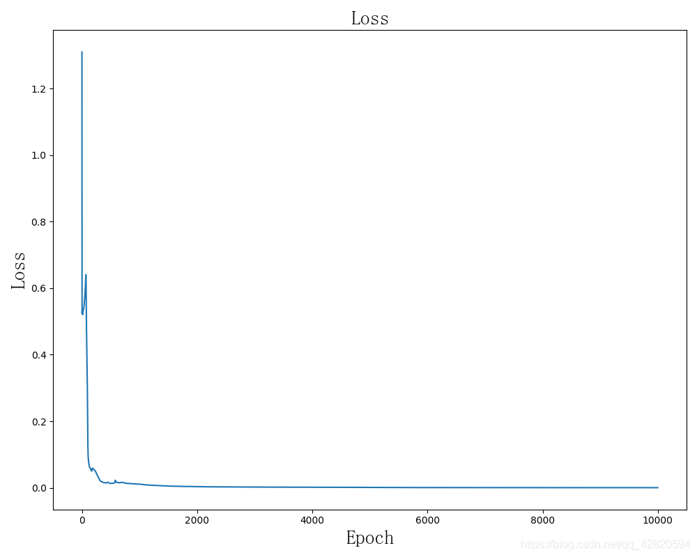

关于权值初始化

不同初始化方法收敛速度分析：

  学习率为0.01。修改初始化的地方在这里：

---

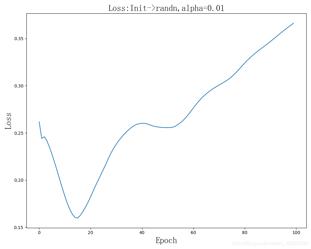
似乎有时候会出现Loss增大的情况，但是随机的，与初始化值和学习率有关。

第一幅图最终结果：epoch:99,loss:0.068638,accrucy : 0.903309

---

效果很差。

epoch:99,loss:0.129023,accrucy : 0.307653

效果有一次很差，我想大胆推断这样初始化的效果都很差，但是这样不科学，我试着改变学习率为0.1，效果有所提升。

epoch:99,loss:0.129075,accrucy : 0.307653

epoch:99,loss:0.003670,accrucy : 0.767322

---

这种初始化方式可见非常糟糕，虽然几乎是线性下降，但是下降速度简直不要太慢。

epoch:0,loss:4.500000,accrucy : 0.103413
epoch:12,loss:4.500000,accrucy : 0.103413
epoch:13,loss:4.500000,accrucy : 0.103930
epoch:499,loss:4.500000,accrucy : 0.105481

注： 偏置b初始化的方式对收敛影响不大，这个读者可以自己试试。

为什么不同的初始化收敛速度不一样？

待续~

关于损失函数

待续~

关于我的感想

  隐含层神经元数量不是越多越好，我以前用PyTroch试过训练和这个网络差不多的有个网络，输入层，输出层和这个神经网络一样，开始隐含层有64和24个神经元，效果含不错，但是我试着改变隐含层神经元的数量使之更多，效果反而不好，并且由于运算量增加，迭代速度大大下降。

  从上面的实验结果看似乎权值初始化的时候使用标准正态分布的随机值会比较好，但这是为什么还值得继续学习。此外似乎偏置b初始化的方式对收敛影响不大，这个读者可以自己试试。

---

  关于学习神经网络，如果你是以实用主义来思考的，那么可能你就只需把机器学习领域的算法了解一遍，学会用框架就可以了。但是这也就只是会用罢了。

  倘如你想要研究这些网络，试图提高它的准确性、收敛速度、预测速度、内存占用、复杂度等等各种性能，以至于创造一种全新的结构、全能的结构、可以组合的结构等等都需要对它们有深入的了解，而不是只会使用框架这种皮毛。其次学习过程也不能囫囵吞枣，要循序渐进，以实践总结理解为主。

---

关于欺骗神经网络，神经网络漏洞

附录

文章资源

手写数字识别全连接神经网络教学Demo：将digits.zip解压到net.py，安装好环境即可运行。

git clone https://github.com/MisakaMikoto128/FCNNeuralNetworkDemoForHandwrittenDigits.git

备份。

参考

[1] 神经网络求导
[2] 常见的损失函数(loss function)总结
[3] 矩阵求导术（上）
[4] 矩阵求导术（下）
[5] 小白都能看懂的softmax详解

链接失效Call我。
github:https://github.com/MisakaMikoto128
个人网站