当前位置:网站首页>Combat readiness mathematical modeling 32 correlation analysis 2
Combat readiness mathematical modeling 32 correlation analysis 2
2022-06-26 14:29:00 【nuist__ NJUPT】
Catalog
One 、 Pearson correlation coefficient
Two 、 Spearman correlation coefficient
3、 ... and 、 Canonical correlation analysis
1- Definition and specific steps
2- Typical cases of correlation analysis 1
3- Typical cases of correlation analysis 2
This section focuses on two types of correlation analysis ,pearson and spearman, They can measure the correlation between two variables , We need to meet different conditions according to the data , Select different correlation coefficients for calculation and analysis , Introduce some details , Personal feelings are more important , Prevent the abuse of correlation analysis . meanwhile , We also discuss the application of canonical correlation analysis , A multivariate linear statistical method mainly used to solve the correlation between two groups of variables .
One 、 Pearson correlation coefficient
Let's take a look at the use requirements of Pearson and Spearman , For Pearson, the variables are required to be continuous data , And the variables have a linear relationship , And the data should obey the normal distribution , And generally, Pearson requires to use the correlation test between fixed distance and fixed distance variables , Sequencing and sequencing variables require Spearman .

Because there are many limitations of Pearson correlation test , We need to verify the restrictions before using , Whether it is a constant distance variable and whether it is continuous can be directly seen , So we first need to test the linearity of the variables , adopt SPSS Draw a matrix scatter , To determine whether there is a linear relationship between variables , There must be a linear relationship , To use the Pearson test .
Let's just look at an example , As follows :

First step : For data , We'd better start with descriptive statistics , This is a good habit , Is to calculate the maximum value of each index , mean value , Standard deviation , Skewness and kurtosis , It can be used SPSS perhaps MATLAB Such as implementation , Of course EXCEL It's fine too , Ha ha ha ha .
SPSS The method of describing statistics is simple , After importing data , Select descriptive statistics , Import variables into , It can be calculated automatically , As shown below .

Of course MATLAB Programming is also very simple , The code is as follows :
clear; clc
load('test_data.mat')
format short g
% Descriptive statistics
Min = min(test) ;
Max = max(test) ;
Mean = mean(test) ;
Median = median(test) ;
Skewness = skewness(test) ; % skewness
Kurtosis = kurtosis(test) ; % kurtosis
Std = std(test) ;
Result = [Min; Max; Mean; Median; Skewness; Kurtosis; Std] ;
disp(' The descriptive statistics are as follows :') ;
disp(Result) ;
The second step , Is the use of SPSS Plot the matrix scatter diagram , The specific operation is as follows , Select graphics -> Old dialog -> Scatter plot -> Matrix three scatter diagram , The matrix scatter diagram drawn is as follows , Of course , The above tabular data is randomly generated , Most normal models have linear relationships .

The third step , Assume that there is a linear relationship between the variables of the above scatter diagram , Now we will calculate the Pearson correlation coefficient , Specifically MATLAB The procedure is as follows , Of course with SPSS It can also be calculated .
% Calculate the Pearson correlation coefficient
R = corrcoef(test) ;
disp(' The Pearson correlation coefficient is as follows :') ;
%xlswrite('D:\r1.xlsx',R) ;
disp(R) ;
We can have a look SPSS The results of Pearson correlation analysis , As follows :
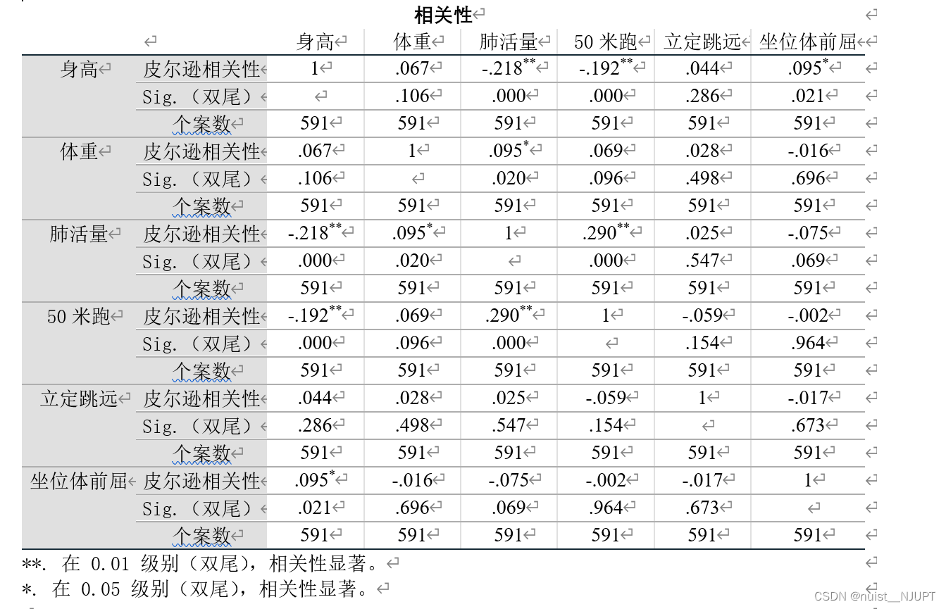
Test the hypothesis of the Pearson correlation coefficient ,p Value test ,p The smaller the value. , The closer the correlation is 1, adopt p It's worth rejecting the original assumption , It shows that Pearson correlation coefficient is significantly different from 0.

Step four , Normal distribution test is required , For large sample data , have access to JB Inspection and QQ Graph test . For small sample data , Use Shapiro - Wilke test .

JB Tested MATLAB The code is as follows , Be careful : This original assumption is a normal distribution , We can't reject the original hypothesis to show that it obeys the normal distribution .
% For large sample data ,n>30 The data of , Normal distribution test , Use JB test , Jacques - Bella test
[h,p] = jbtest(test(:,1),0.05) ; % Check whether the data in the first column is normally distributed
% Check the data of all columns with a loop
n_c = size(test, 2) ;
H = zeros(1,6) ;
P = zeros(1,6) ;
for i = 1 : n_c
    [h,p] = jbtest(test(:,i), 0.05) ;
    H(i) = h ;
    P(i) = p ;
end
% If H be equal to 1 It means rejecting the original hypothesis ,P<0.5 You can reject the original hypothesis
disp('H The values are as follows :') ;
disp(H) ;
disp('P The values are as follows :') ;
disp(P) ;
You can also use it QQ Fig. test whether the large sample obeys the normal distribution , But this only depends on the trend , Not accurate enough .

Draw... In this question QQ The code of the figure is as follows :
subplot(2,3,1) ;
qqplot(test(:,1)) ;
title(' Height data and standard normal QQ chart ') ;
xlabel(' Standard normal number ') ;
ylabel(' Enter the number of samples ') ;
subplot(2,3,2);
qqplot(test(:,2)) ;
title(' Body weight data and standard normal QQ chart ') ;
xlabel(' Standard normal number ') ;
ylabel(' Enter the number of samples ') ;
subplot(2,3,3) ;
qqplot(test(:,3)) ;
title(' Vital capacity data and standard normal QQ chart ') ;
xlabel(' Standard normal number ') ;
ylabel(' Enter the number of samples ') ;
subplot(2,3,4);
qqplot(test(:,4)) ;
title('50 Meter run data and standard normal QQ chart ') ;
xlabel(' Standard normal number ') ;
ylabel(' Enter the number of samples ') ;
subplot(2,3,5) ;
qqplot(test(:,5)) ;
title(' Standing long jump data and standard normal QQ chart ') ;
xlabel(' Standard normal number ') ;
ylabel(' Enter the number of samples ') ;
subplot(2,3,6);
qqplot(test(:,6)) ;
title(' The forward flexion data of sitting posture are compared with that of standard normal QQ chart ') ;
xlabel(' Standard normal number ') ;
ylabel(' Enter the number of samples ') ;
QQ The graph is as follows , If it approximates to a straight line , It shows that the distribution is normal , As follows :

Use Shapiro for small sample data - Whether Wilke test obeys normal distribution ,SPSS Implementation steps , As follows :

The inspection results are as follows , If the significance is less than 0.05, Reject the null hypothesis , It means that the normal distribution is not obeyed .

Pearson test , complete MATLAB The code is as follows :
clear; clc
load('test_data.mat')
format short g
% Descriptive statistics
Min = min(test) ;
Max = max(test) ;
Mean = mean(test) ;
Median = median(test) ;
Skewness = skewness(test) ; % skewness
Kurtosis = kurtosis(test) ; % kurtosis
Std = std(test) ;
Result = [Min; Max; Mean; Median; Skewness; Kurtosis; Std] ;
disp(' The descriptive statistics are as follows :') ;
disp(Result) ;

% Before calculating the Pearson coefficient , You need to make a scatter plot , Observe whether the two groups of variables have a linear relationship according to the scatter diagram
% We can use SPSS Achieve the above operation , Operate in the graphics options


% For large sample data ,n>30 The data of , Normal distribution test , Use JB test , Jacques - Bella test
[h,p] = jbtest(test(:,1),0.05) ; % Check whether the data in the first column is normally distributed
% Check the data of all columns with a loop
n_c = size(test, 2) ;
H = zeros(1,6) ;
P = zeros(1,6) ;
for i = 1 : n_c
    [h,p] = jbtest(test(:,i), 0.05) ;
    H(i) = h ;
    P(i) = p ;
end
% If H be equal to 1 It means rejecting the original hypothesis ,P<0.5 You can reject the original hypothesis
disp('H The values are as follows :') ;
disp(H) ;
disp('P The values are as follows :') ;
disp(P) ;

% For small sample data, Shapiro can be used ‐ Whether the Wilke test is a normal distribution
% It can be used SPSS Realization


% Of course, there is another way to test whether the distribution is normal Q-Q chart , Of course, this method requires a large amount of data , And just be able to see the trend
subplot(2,3,1) ;
qqplot(test(:,1)) ;
title(' Height data and standard normal QQ chart ') ;
xlabel(' Standard normal number ') ;
ylabel(' Enter the number of samples ') ;
subplot(2,3,2);
qqplot(test(:,2)) ;
title(' Body weight data and standard normal QQ chart ') ;
xlabel(' Standard normal number ') ;
ylabel(' Enter the number of samples ') ;
subplot(2,3,3) ;
qqplot(test(:,3)) ;
title(' Vital capacity data and standard normal QQ chart ') ;
xlabel(' Standard normal number ') ;
ylabel(' Enter the number of samples ') ;
subplot(2,3,4);
qqplot(test(:,4)) ;
title('50 Meter run data and standard normal QQ chart ') ;
xlabel(' Standard normal number ') ;
ylabel(' Enter the number of samples ') ;
subplot(2,3,5) ;
qqplot(test(:,5)) ;
title(' Standing long jump data and standard normal QQ chart ') ;
xlabel(' Standard normal number ') ;
ylabel(' Enter the number of samples ') ;
subplot(2,3,6);
qqplot(test(:,6)) ;
title(' The forward flexion data of sitting posture are compared with that of standard normal QQ chart ') ;
xlabel(' Standard normal number ') ;
ylabel(' Enter the number of samples ') ;


% Calculate the Pearson correlation coefficient
R = corrcoef(test) ;
disp(' The Pearson correlation coefficient is as follows :') ;
%xlswrite('D:\r1.xlsx',R) ;
disp(R) ;
Two 、 Spearman correlation coefficient
Let's take another look at this comparison , When we find that it is not difficult to use Pearson correlation coefficient test , Then we can consider using Spearman test , As follows :

Use MATLAB and SPSS We can find the Spearman correlation coefficient , Given this time MATLAB Code ,SPSS Read another blog about correlation analysis .
clear; clc
load('test_data.mat')
format short g

% Calculate Spearman correlation coefficient
R = corr(test, 'type', 'Spearman') ;
disp(' Spearman correlation coefficient is as follows :') ;
disp(R) ;
For Spearman's hypothesis test ,p Less than 0.05, You can reject the original hypothesis , Then explain and 0 There are significant differences , Otherwise, it is not difficult to reject the original assumption .

3、 ... and 、 Canonical correlation analysis
1- Definition and specific steps
General correlation analysis is used to analyze the correlation between two variables , If we need to consider the correlation between two sets of variables , Canonical correlation analysis .
We can first look at the idea of canonical correlation analysis , In fact, it is similar to dimensionality reduction , Is the linear combination of multiple variables , Form a comprehensive variable , Solving the correlation between comprehensive variables .

We use SPSS Perform canonical correlation analysis , Need to use SPSS24 Above version , As follows , First import the data :

Then the data is checked , Normal data are scaled , As shown below .

Then carry out canonical correlation analysis , Import two groups of variables respectively , as follows :


Next , The results of the analysis can be everywhere you want .

2- Typical cases of correlation analysis 1
Carry out canonical correlation analysis on the following body index data , Refer to the above for specific steps .

The results of my analysis are as follows :


3- Typical cases of correlation analysis 2
We want to explore the relationship between the views of viewers and insiders on some TV programs ?
Audience rating comes from low education (led)、 Highly educated (hed) And the Internet (net) Investigate three , They form the first set of variables ;
The scores of the insiders come from artists including actors and directors (arti)、 issue (com) With the industry
Head of Department (man) Three , Form the second set of variables .
Follow the above typical correlation analysis steps , My analysis results are as follows :


边栏推荐
- (improved) bubble sorting and (improved) cocktail sorting
- Record: why is there no lightning 4 interface graphics card docking station and mobile hard disk?
- Related knowledge of libsvm support vector machine
- Sword finger offer 10 Ⅰ 10Ⅱ. 63 dynamic planning (simple)
- Practice with the topic of bit operation force deduction
- [wc2006] director of water management
- CF676C Vasya and String
- 年薪50万是一条线,年薪100万又是一条线…...
- 9項規定6個嚴禁!教育部、應急管理部聯合印發《校外培訓機構消防安全管理九項規定》
- Leaflet loading ArcGIS for server map layers
猜你喜欢

BP neural network for prediction

Sword finger offer 40.41 Sort (medium)

Eigen(3):error: ‘Eigen’ has not been declared

从Celsius到三箭:加密百亿巨头们的多米诺,史诗级流动性的枯竭

9 regulations and 6 prohibitions! The Ministry of education and the emergency management department jointly issued the nine provisions on fire safety management of off campus training institutions

量化框架backtrader之一文读懂observer观测器

登录认证服务

Related knowledge of libsvm support vector machine

服务器创建虚拟环境跑代码
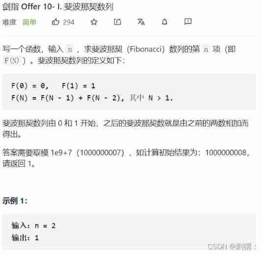
Sword finger offer 10 Ⅰ 10Ⅱ. 63 dynamic planning (simple)
随机推荐
Knowledge about adsorption
C language | the difference between heap and stack
Eigen(3):error: ‘Eigen’ has not been declared
MySQL | basic commands
(improved) bubble sorting and (improved) cocktail sorting
2021-10-29 atcoder ABC157——B - Bingo
Pychar remotely connects to the server to run code
通俗语言说BM3D
Is it safe to open a securities account? Is there any danger
服务器创建虚拟环境跑代码
常用控件及自定义控件
Why is there always a space (63 or 2048 sectors) in front of the first partition when partitioning a disk
方程推导:二阶有源带通滤波器设计!(下载:教程+原理图+视频+代码)
C language ---getchar() and putchar()
Server create virtual environment run code
Sword finger offer 05.58 Ⅱ string
ThreadLocal巨坑!内存泄露只是小儿科...
wptx64能卸载吗_win10自带的软件哪些可以卸载
When drawing with origin, capital letter C will appear in the upper left corner of the chart. The removal method is as follows:
H5关闭当前页面,包括微信浏览器(附源码)