Illustration of ONEFLOW's learning rate adjustment strategy

writing ｜ Li Jia

1、 background

Learning rate adjustment strategies （learning rate scheduler）, In fact, it's not difficult to take each one out alone , But because there are many methods , It's easy to get confused when you read the document ,  With OneFlow v0.7.0 For example ,oneflow.optim.lr_scheduler The module contains 14 Strategies .

Is there a better way to learn ？ For example, visualize the change process of learning rate , here , It suddenly occurred to me that Convolution Arithmetic This classic project , The author will introduce all kinds of CNN Convolution operation to gif Form show , Be clear at a glance .

therefore , There is this article , Visualize learning rate adjustment strategies , Here are two examples （ConstantLR and LinearLR）：

I have managed the visualization code separately in Hugging Face Spaces and Streamlit Cloud, You can choose any link to visit , Then adjust the parameters freely , Feel the changing process of learning rate .

• https://huggingface.co/spaces/basicv8vc/learning-rate-scheduler-online

• https://share.streamlit.io/basicv8vc/scheduler-online

2、 Learning rate adjustment strategies

Learning rate is the most important parameter in training neural network （ One of ）, At present, it has been accepted that the dynamic learning rate adjustment strategy is used to replace the fixed learning rate , Various learning rate adjustment strategies emerge in endlessly , So let's do that

OneFlow v0.7.0

For example , Learn some common strategies .

Base class LRScheduler

LRScheduler(optimizer: Optimizer, last_step: int = -1, verbose: bool = False) Is the base class for all learning rate schedulers , Initialization parameters last_step and verbose You don't usually need to set it , The former is mainly related to checkpoint relevant , The latter is every time step()  Print the learning rate when calling , It can be used for  debug.LRScheduler The most important method in step(), The function of this method is to modify the initial learning rate set by the user , Then apply to the next Optimizer.step().

Some materials will say LRScheduler according to epoch or iteration/step To adjust the learning rate , Both statements are OK , actually ,LRScheduler I don't know how many times I have been training epoch Or the number iteration/step, Only calls are recorded step() The number of times （last_step）, If each epoch Call once , That's the basis epoch To adjust the learning rate , If each mini-batch Call once , That's the basis iteration To adjust the learning rate . To train Transformer The model, for example , Need to be in every iteration call step().

Simply speaking ,LRScheduler According to the adjustment strategy itself 、 The current call step() The number of times （last_step） And the initial learning rate set by the user to get the learning rate at the next gradient update .

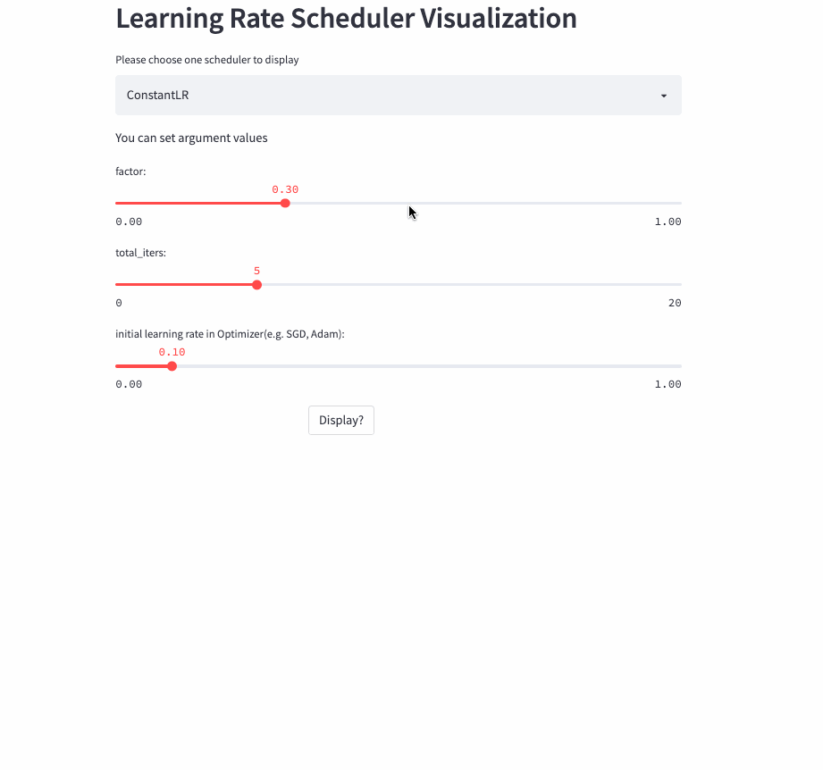
ConstantLR

oneflow.optim.lr_scheduler.ConstantLR(
 optimizer: Optimizer,
 factor: float = 1.0 / 3,
 total_iters: int = 5,
 last_step: int = -1,
 verbose: bool = False,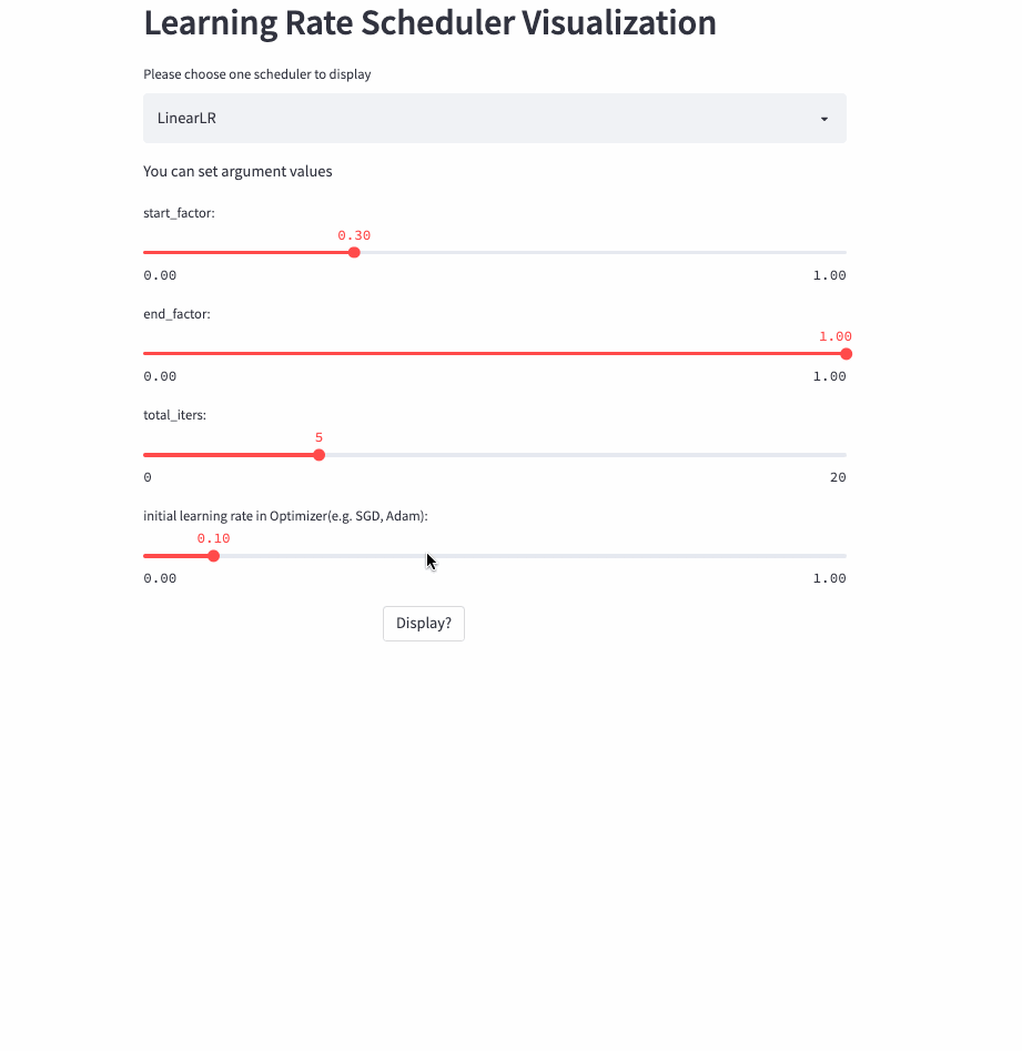
)

ConstantLR Similar to the fixed learning rate , The only difference is that before total_iters, The learning rate is the initial learning rate  * factor.

Be careful ： because factor Value [0, 1], So this is a strategy of increasing learning rate .

ConstantLR

LinearLR

oneflow.optim.lr_scheduler.LinearLR(
 optimizer: Optimizer,
 start_factor: float = 1.0 / 3,
 end_factor: float = 1.0,
 total_iters: int = 5,
 last_step: int = -1,
 verbose: bool = False,
)

LinearLR It is similar to the fixed learning rate , The only difference is that before total_iters, Learn to take the lead in increasing or decreasing linearly , And then fixed to the initial learning rate  * end_factor.

Be careful ： The learning rate is in the top total_iters It's incremental or Decrement by start_factor and end_factor Size decides .

LinearLR

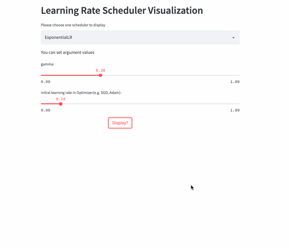
ExponentialLR

oneflow.optim.lr_scheduler.ExponentialLR(
 optimizer: Optimizer,
 gamma: float,
 last_step: int = -1,
 verbose: bool = False,
)

The learning rate decays exponentially , Of course, you can also gamma Set to >1, Increase exponentially , But no one is willing to do so .

ExponentialLR

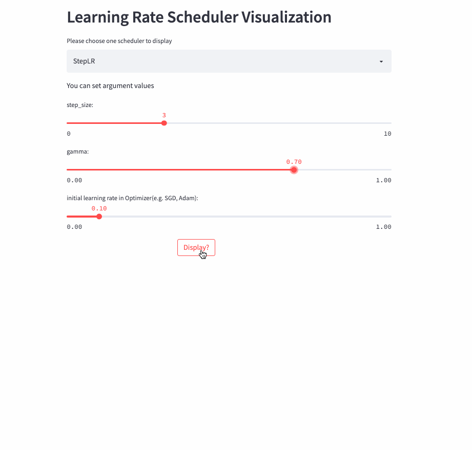
StepLR

oneflow.optim.lr_scheduler.StepLR(
 optimizer: Optimizer,
 step_size: int,
 gamma: float = 0.1,
 last_step: int = -1,
 verbose: bool = False,
)

StepLR and ExponentialLR almost , The difference is whether each call step() To adjust the learning rate , But every step_size Only once .

StepLR

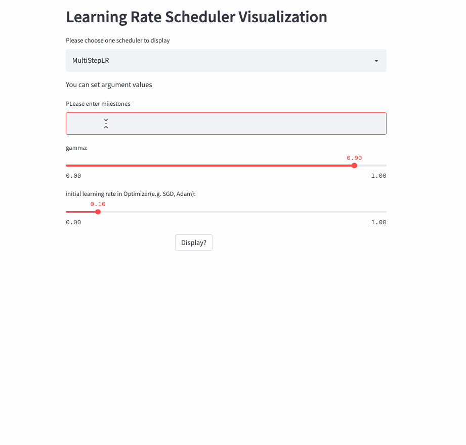
MultiStepLR

oneflow.optim.lr_scheduler.MultiStepLR(
 optimizer: Optimizer,
 milestones: list,
 gamma: float = 0.1,
 last_step: int = -1,
 verbose: bool = False,
)

StepLR every other step_size Just adjust the learning rate once , and MultiStepLR According to the user specified milestones Adjustment , hypothesis milestones yes [2, 5, 9], stay [0, 2) yes lr, stay [2, 5) yes lr * gamma, stay [5, 9) yes lr * (gamma **2), stay [9, ) yes lr * (gamma **3).

MultiStepLR

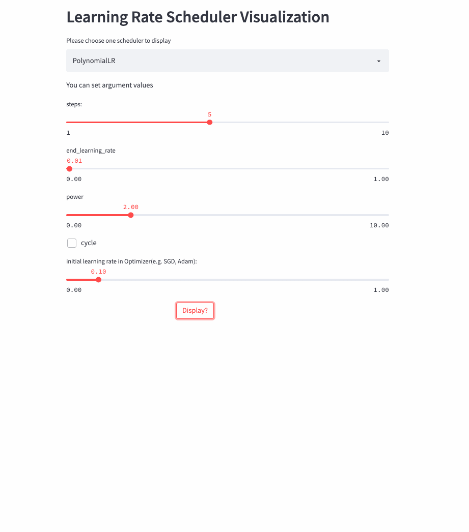
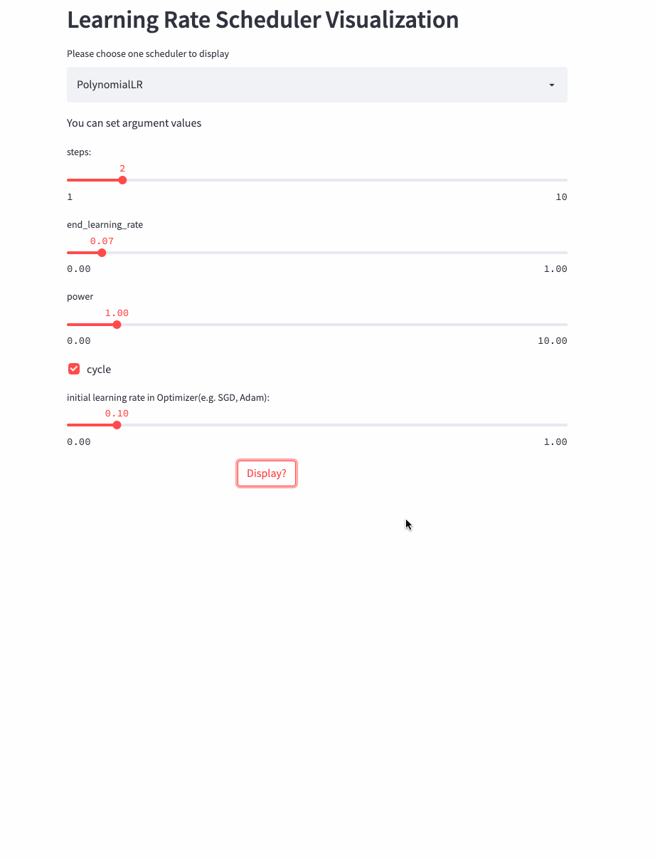
PolynomialLR

oneflow.optim.lr_scheduler.PolynomialLR(
 optimizer,
 steps: int,
 end_learning_rate: float = 0.0001,
 power: float = 1.0,
 cycle: bool = False,
 last_step: int = -1,
 verbose: bool = False,
)

The previous learning rate adjustment strategy is nothing more than linear or exponential ,PolynomialLR Then adjust according to the polynomial , First look at cycle Parameters , The default is False, In this case, the learning rate is fixed after the polynomial decay , The formula is as follows ：

notes ： Formula decay_batch Namely steps,current_batch It's the latest last_step.

If cycle yes True, It's a little more complicated , Similar to steps Change for the period , Decay from a maximum learning rate to end_learning_rate, The maximum learning rate of each cycle also decreases gradually , The formula is as follows ：

PolynomialLR

look down cycle=True Example ,

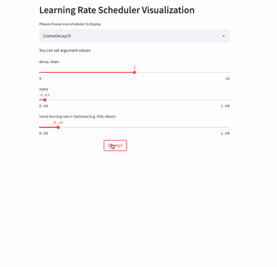
CosineDecayLR

oneflow.optim.lr_scheduler.CosineDecayLR(
 optimizer: Optimizer,
 decay_steps: int,
 alpha: float = 0.0,
 last_step: int = -1,
 verbose: bool = False,
)

before decay_steps Step , The learning rate is determined by lr The cosine decays to lr * alpha, Then fix it as lr*alpha.

notes ：CosineDecayLR To align TensorFlow Medium CosineDecay.

CosineAnnealingLR

oneflow.optim.lr_scheduler.CosineAnnealingLR(
 optimizer: Optimizer,
 T_max: int,
 eta_min: float = 0.0,
 last_step: int = -1,
 verbose: bool = False,
)

CosineAnnealingLR and CosineDecayLR It's like , The difference is that the former includes not only the process of cosine attenuation , It can also include cosine increase , before T_max Step , The learning rate is determined by lr The cosine decays to eta_min,  If cur_step > T_max, Then the cosine is increased to lr, Repeat the process over and over again .

CosineAnnealingLR

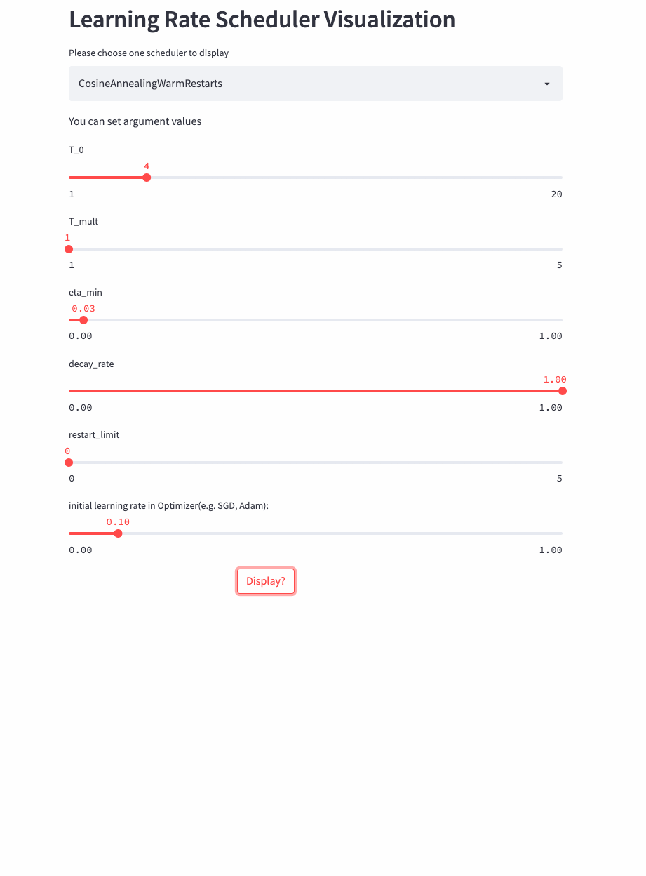
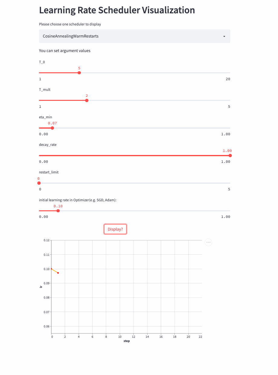
CosineAnnealingWarmRestarts

oneflow.optim.lr_scheduler.CosineAnnealingWarmRestarts(
 optimizer: Optimizer,
 T_0: int,
 T_mult: int = 1,
 eta_min: float = 0.0,
 decay_rate: float = 1.0,
 restart_limit: int = 0,
 last_step: int = -1,
 verbose: bool = False,
)

The three above Cosine dependent LRScheduler From the same paper （SGDR: Stochastic Gradient Descent with Warm Restarts）, There are many parameters , First of all to see T_mul, If T_mul=1, Then the learning rate changes periodically , The size of the period is T_0, That is, the number of steps from the maximum learning rate to the minimum learning rate (steps), Note that if decay_rate<1, Then the maximum learning rate and the minimum learning rate of each cycle are declining , The first cycle consists of lr Start decaying , The second cycle consists of lr * decay_rate Start decaying , The third cycle consists of lr * (decay_rate ** 2) Start decaying .

If T_mult>1, Then the learning rate does not change in an equal period , The size of each cycle is the size of the previous cycle T_mult, The first cycle is T_0, The second cycle is T_0 * T_mult, The third cycle is  T_0 * T_mult * T_mult.

Look again. restart_limit, The default value is 0, That's the process above , If >0, The physical meaning is the number of cycles , Assuming that 3, Then there are only three decays from maximum to minimum , Then the learning rate has been eta_min, It doesn't change periodically .

Let's have a look T_mult=1 Example , here decay_rate=1,

T_mult=1, decay_rate=1

Another look T_mult=1,decay_rate=0.5 Example , Note that this combination is not commonly used .

T_mult=1, decay_rate=0.5

Look again. T_mult >1 Example ,

Last , Another look restart_limit != 0 Example ,

3、 Combined scheduling strategy

All the above are single learning rate scheduling strategies , Let's look at several learning rate combined scheduling strategies , Like training Transformer frequently-used Noam scheduler You need to increase linearly and then decay exponentially , Can pass LinearLR and ExponentialLR Combine to get . It can also be used directly LambdaLR Incoming learning rate change function .

LambdaLR

oneflow.optim.lr_scheduler.LambdaLR(optimizer, lr_lambda, last_step=-1, verbose=False)

LambdaLR It can be said to be the most flexible strategy , Because the specific method is based on the function lr_lambda Designated . Such as the implementation Transformer Medium Noam Scheduler：

def rate(step, model_size, factor, warmup):
 """
 we have to default the step to 1 for LambdaLR function
 to avoid zero raising to negative power.
 """
 if step == 0:
 step = 1
 return factor * (
 model_size ** (-0.5) * min(step ** (-0.5), step * warmup ** (-1.5))
 )


model = CustomTransformer(...)
optimizer = flow.optim.Adam(
 model.parameters(), lr=1.0, betas=(0.9, 0.98), eps=1e-9
)
lr_scheduler = LambdaLR(
 optimizer=optimizer,
 lr_lambda=lambda step: rate(step, d_model, factor=1, warmup=3000),
)

Be careful ：OneFlow Of Graph Mode does not support LambdaLR.

SequentialLR

oneflow.optim.lr_scheduler.SequentialLR(
 optimizer: Optimizer,
 schedulers: Sequence[LRScheduler],
 milestones: Sequence[int],
 interval_rescaling: Union[Sequence[bool], bool] = False,
 last_step: int = -1,
 verbose: bool = False,
)

Support the transfer of multiple LRScheduler, Every LRScheduler The scope of action of （step range） from milestones Appoint , Let's see interval_rescaling This parameter , The default is False, The purpose is to make two adjacent scheduler The learning rate is relatively smooth when connecting , such as milestones=[5], When last_step=5 when , the second schduler From last_step=5 Start calculating the new learning rate , And so last_step=4（ Previous scheduler Calculate the learning rate ） There will be no big difference in the learning rate , and interval_rescaling=True when , Then this scheduler Of last_step from 0 Start .

WarmupLR

oneflow.optim.lr_scheduler.WarmupLR(
 scheduler_or_optimizer: Union[LRScheduler, Optimizer],
 warmup_factor: float = 1.0 / 3,
 warmup_iters: int = 5,
 warmup_method: str = "linear",
 warmup_prefix: bool = False,
 last_step=-1,
 verbose=False,
)

WarmupLR yes SequentialLR Subclasses of , Contains two LRScheduler, And the first one is either ConstantLR, Or LinearLR.

ChainedScheduler

oneflow.optim.lr_scheduler.ChainedScheduler(schedulers)

The combined scheduling strategy mentioned above , In every one of them step, only one LRScheduler Play a role , and ChainedScheduler, In every one of them step When calculating the learning rate , be-all LRScheduler All involved , It's like a pipe （pipeline）

lr ==> LRScheduler_1 ==> LRScheduler_2 ==> ... ==> LRScheduler_N

ReduceLROnPlateau

oneflow.optim.lr_scheduler.ReduceLROnPlateau(
 optimizer,
 mode="min",
 factor=0.1,
 patience=10,
 threshold=1e-4,
 threshold_mode="rel",
 cooldown=0,
 min_lr=0,
 eps=1e-8,
 verbose=False,
)

All the above mentioned LRScheduler Are based on the current step To calculate the learning rate , In the process of model training , We are most concerned about the indicators on the training set and the verification set , Can we use these indicators to guide the change of learning rate ？ You can use ReduceLROnPlateau, If there are multiple indicators step Have not changed significantly , The learning rate decays linearly .

optimizer = flow.optim.SGD(model.parameters(), lr=0.1, momentum=0.9)
scheduler = flow.optim.lr_scheduler.ReduceLROnPlateau(optimizer, 'min')
for epoch in range(10):
 train(...)
 val_loss = validate(...)
 #  Be careful , This step should be done at validate() Then call .
 scheduler.step(val_loss)

4、 practice

If you see here, you still have a sense of meaning , It's better to practice , The following is my rewriting based on the official image classification example CIFAR-100 Example , You can set different learning rate scheduling strategies to feel the difference

• https://github.com/basicv8vc/oneflow-cifar100-lr-scheduler

（ This document is issued after authorization , original text ：https://zhuanlan.zhihu.com/p/520719314&nbsp;）

Everyone else is watching

• Overview of deep learning

• The journey of an operator in the framework of deep learning

• The optimal parallel strategy of distributed matrix multiplication is derived by hand

• Train a large model with hundreds of billions of parameters , Four parallel strategies are indispensable

• Reading Pathways（ Two ）： The next step forward is OneFlow

• About concurrency and parallelism ,Go and Erlang My father is mistaken ？

• OneFlow v0.7.0 Release ：
  New distributed interface ,LiBai、Serving Everything

Welcome to download experience  OneFlow v0.7.0  The latest version ：

https://github.com/Oneflow-Inc/oneflow/