ADC acquisition noise and comparison between RMS filter and Kalman filter

    For a while, the author was doing a PT100 The conditioning circuit of thermal resistance adopts , Use a constant current source to measure the resistance of the thermal resistance . For the convenience of collection , take 0.3mA The current of is connected PT100 Put... Directly ADC The input terminal is connected to PT100 Both ends . When the temperature is output later, the data is very chaotic . Access to information is inspired , Use to find the effective value of the signal （ Root mean square value ） Method to filter .

• ADC sampling 、 Constant current source

    ADC It uses STM32F10x Inside the series 12 position ADC. The current value of the constant current source is 0.3mA.

• PT100 Thermal resistance

    PT100 It's below zero , The resistance value is 100Ω Thermal resistance of , The temperature characteristic curve is shown in the figure 1

chart 1：PT100 Temperature characteristic curve

    Basically, in -200—600 There is a linear relationship between temperature and resistance . Therefore, measurement PT100 One way to measure resistance is to give PT100 Connect a constant current source , Then measure the voltage at both ends and then calculate PT100 Resistance value .

• Noise analysis

    Power on the circuit （ The power supply adopts two sections 18650 Series connection ,AMS1115-3.3V Voltage reduction and stabilization ） Connect both ends of the thermal resistance to the oscilloscope （ Input impedance 1MΩ） Pictured 2.Single once , Then, all the sampling data in the interface are processed FFT（ The fast Fourier transform ） Get the picture 3、 chart 4. It is not difficult to see that the noise mainly comes from 1Mhz And some Gaussian white noise .

                                                                                    chart 2： The original signal

                                                                                          chart 3：FFT

                                                                                            chart 4：FFT

 

• Root mean square noise removal

                                                                          

    To find the root mean square value of a signal is actually to find the effective value of the signal （RMS） That is, the mean square of the signal is redistributed .ADC Sampling frequency is 10Khz. Every time 100 Data to calculate . The calculated data is output by the serial port , See the picture :6、 chart 7.（C See the program for the code 1）

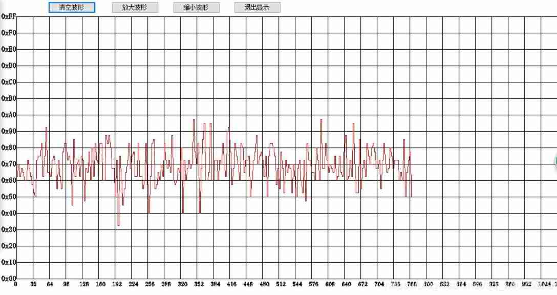
                                                                                  chart 5： Serial port outputs raw data

                                                                                    chart 6： Filter data

                                                                              chart 7： to PT100 Heating temperature

• First order low pass filter

                                                                        y(n) = q*x(n) + (1-q)*y(n-1)

    in Y（n） For export ,x（n） For input . among Q take 0.5 The input waveform is shown in Figure 8.（C See the program for the code 2）

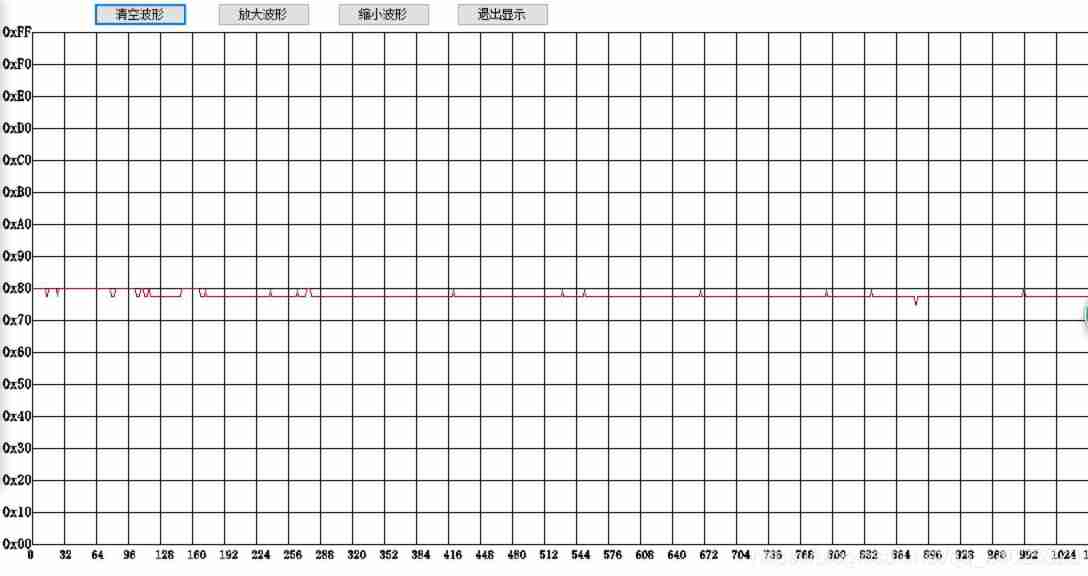
                                                                        chart 8： Add the first-order low-pass filter serial port output

 

• kalman wave filtering

    The first step is to import the data MATLAB, Draw the raw data curve . See the picture 9.. Make the data as Kalman filter observation matrix . Put the data of t-2 To t The mean value of the time is used as the speculative matrix （ See additional code for details ）. Finally, the Kalman output is made into a moving average . Kalman output model （ Blue ） See the picture 10.（matlab See the program for the code 3）

                                                                              chart 9：MATLAB Import raw data

                                                                            chart 10： Raw data and filtered data

• summary ：

    A large part of the reason for the noise is that the digital and analog are not separated when drawing the circuit board .Kalman Filtering algorithm is a filtering algorithm based on time domain . The author thinks that the Gaussian white noise in this circuit mainly comes from the interference of power supply and digital signal to analog signal . As far as this circuit is concerned, it is an effective method to find the root mean square value of the signal . The author has limited knowledge , If there are mistakes, please correct them .

 

• Program 1

unsigned int disposePT100v()
{
	unsigned char i;
	double dData[100];
	double dSum;
	for(i=0;i<100;i++)
	{
		dData[i] = g_iADC[0];// obtain ADC data 
		dSum +=pow(dData[i],2);// Do the sum of squares 
		delay_us(100);
	}
	dSum /= 100;// Calculating mean 
	dSum = sqrt(dSum);// prescribing 
	return (unsigned int)dSum*3300/4096;//mv Voltage value 
}

• Program 2

unsigned int lowV(unsigned int com)
{
	static unsigned int iLastData;
	unsigned int iData;
	double dPower=0.5;
	iData = (com*dPower)+(1-dPower)*iLastData;// Calculation 
	iLastData = iData;//jilu 
	return iData;// Return the data 
}

• Program 3

clear
clc
ydata=textread('a123.txt','%s');%% Import data 
cData = hex2dec(ydata);% Convert to 10 Hexadecimal data 

%t-1 The output of the time is taken as the estimated value of the system at this time    Optimal deviation （ initial value ）g_zer   Speculative error ( initial value )g_ter   Measured value deviation （ initial value ）g_cer
% Measurement results ( matrix ) ner1    Conjecture （ matrix ）ner2  (end)
g_zer = 5;%% Initial value of optimal deviation 
g_ter = 3;%% Guess the initial value of deviation 
g_cer = 2;%% Measure the initial value of deviation 
kdata = 0;
for i=1:5792%% iteration 5000 Time 
    ner1 = cData(i);
    if i>3
        ner2 = (cData(i-2)+cData(i-1)+cData(i))/3;%%t-2 Moment to t The average value of time is taken as t The estimated value of time 
    else
        ner2 = kdata;
    end
    if g_zer>g_ter
    g_er = sqrt((g_zer^2)-(g_ter^2));% Calculate this error 
    else
    g_er = sqrt((g_ter^2)-(g_zer^2));% Calculate this error 
    end
    kk = sqrt((g_er^2)/((g_er^2)+(g_cer^2)));% Calculate Kalman gain 
    kdata = ner1+kk*(ner2-ner1);% Update Kalman output 
    g_zer = ((1-kk)*g_ter^2)^0.5;% Calculate the optimal deviation 
    cKdata(i) = kdata;
end
%%%%%%% moving average %%%%%%%%%%
t = 1:5792;
a = 0;
b = 0;
pKdata = zeros(1,5792);
for i=1:5700
    for j=1:50
        a = a + cKdata(i+j);
    end
    b = a/50;%% Averaging 
    a = 0;
    pKdata(i)=b;
end
plot(t,cData,'R',t,cKdata,'G',t,pKdata,'B');