当前位置：网站首页>Comprehensive introduction to Simulink solver

This paper gives a comprehensive introduction to Simulink All aspects of the solver . Finally, a simple example is given to illustrate the influence of the configuration of the solver on the simulation results .

2. Simulink solver

2.1 Simulink simulation process

Simulink The execution of the model is carried out in several stages . The first step is the initialization phase , At this stage ,Simulink Merge library model blocks into the model , Determine the transfer width 、 Data type and sampling time , Calculate block parameters , Determine the execution order of the blocks , And allocate memory . then ,Simulink Enter into “ Simulation loop ”, The simulation time of each cycle is advanced by one simulation “ Time step ”, Time step （time step） Is the time interval at which the calculation occurs , The size of this time interval is called step . During each simulation time step ,Simulink Execute each block in the model in sequence according to the block execution order determined in the initialization phase . For each block ,Simulink Call the function to calculate the status of the block at the current sampling time , Derivative and output . So again and again , Continue until the end of the simulation . The process of calculating the state of a model in this way is called Solution Model .

2.2 Simulink Solver classification

No model solving method can be applied to all systems .Simulink Provides a set of programs , be called solver . Each solver represents a specific model solving method .

The solver uses a numerical method to solve a set of ordinary differential equations representing the model . By this calculation , It determines the time for the next simulation step . In the process of solving this initial value problem , The solver also meets the accuracy requirements you specify .

Mathematicians have developed a variety of numerical integration methods to solve ordinary differential equations that represent the continuous state of dynamic systems (ODE). This paper provides a comprehensive set of constant step size and variable step size continuous solvers , Each of these solvers implements a specific ODE solution （ see also Compare solvers ）. In the model configuration parameter solver Pane, select solver .

MATLAB and Simulink All solvers provided follow a similar naming convention ：ode Followed by twoorthree numbers （ Represents the order of the solver ）. Some solvers can solve rigid differential equations , The methods they use are s、t or tb postfix notation .

Simulink Solvers can be classified into two categories based on the type of calculation step ： Variable step size solver and fixed step size solver . Based on the model state classification, it can be divided into ： Continuous and discrete solvers . It is further subdivided into ： Implicit solution and explicit solution 、 Single step solution, multi-step solution, single order solution and variable order solution .

（1） Fixed step size and variable step size solvers

The simulation step of the fixed step solver is fixed , There is no error control mechanism ; The variable step size solver needs to calculate the simulation step size in the simulation process , By increasing the / Reduce the step size to meet the set error tolerance . When generating real-time operation code , A fixed step solver must be used , If you do not plan to configure model code generation , The choice of solver depends on the characteristics of the model and the simulation speed 、 Accuracy and other requirements . Usually , Variable step size solver can reduce simulation time , The smaller the step size is, the smaller the step size is , The higher the simulation accuracy , Therefore, under the same simulation accuracy requirements , When the fixed step solver is used for simulation , The minimum step size in the variable step size solver must be used in the whole simulation process .

（2） Continuous and discrete solvers

There are continuous and discrete solvers in both fixed and variable step size solvers . Both continuous and discrete solvers rely on modules to calculate all discrete state values . The module that defines the discrete state is responsible for calculating the discrete state value at each sampling time point , The continuous solver calculates the state value of the module that defines the continuous state through numerical integration . When selecting a solver , You must first determine whether a discrete solver is required in the model . If there is no continuous state module in the model ,Simulink The discrete solver is automatically selected （ Even if it is set to use the continuous solver ）, If there is a continuous state model, a continuous solver must be used .

（3） Explicit and implicit solvers

The application of implicit solver mainly solves the rigidity problem in the model , Explicit solvers are used to solve nonrigid problems . for example , In the control system , The response of control components is fast changing , With a small time constant , However, the controlled object usually has large inertia 、 Slowly changing , Has a large time constant . Systems with very different time scales are usually referred to as rigid systems , Popular speaking , That is, the system contains time fast and time slow components （ Systems with both small and large time constants ）. The rigid system has a very large resilience, which makes the disturbance of fast changing components attenuate very quickly , When integrating such a system numerically , Once the fast component disappears, it is desirable to select an appropriate time step to calculate the slow component . So the essence of the rigid system is that the solution to be calculated is slow change , But there are disturbances that decay rapidly , The occurrence of such disturbances complicates the numerical calculation of slowly varying solutions . therefore , The oscillation phenomenon in the system , Implicit solution is far more stable than explicit solution , But the computational cost is larger than the explicit solution , It needs to be utilized at each step of the simulation Newton-like Method to calculate the resulting Jacobian （Jacob） Matrix and algebraic equations . In order to reduce the computational cost ,Simulink The parameters for calculating Jacobian method are provided , Improve simulation performance .

（4） Single and multi-step solvers

stay Simulink Single step and multi-step solvers are provided in the solution library . One step solution is to calculate the current moment of the system y(tn), Need to take advantage of the previous moment y(tn-1) And in tn-1 And tn Differential quantity between multiple time points （ These points in time are called microsteps ）; The multi-step solver is to calculate the value of the current time by using the value of the previous time of the system .Simulink An explicit multistep solver is provided ode113 And an implicit multistep solver ode15s, Both are variable step solvers .

（5） Variable order solver

Simulink Two variable order solvers are provided ,ode15s The solver uses 1 Step to 5 Step simulation ;ode113 application 1 Step to 13 rank . about ode15s The highest order can be set .

2.3 Simulink Simulation parameter setting interface

Solver panel ：

(1) Simulation time setting ：

Start time Starting time ： The simulation and generated code are double precision values , Unit second ; The parameter name is StartTime, Parameter type is string.

Stop time End time ： The simulation and generated code are double precision values , Unit second ; The parameter name is StopTime, Parameter type is string; This value should not be less than Start time( If equal , Then only run one step ), It can be set to infinity inf.

(2) Solver settings ： Different solvers , The specific setting parameters are also different , This refers to the common part of the description .

The configuration parameters for the variable step solver include the following ：

Solver

Max step size： Set the maximum step size , Default is auto, It is the time course of simulation 1/50; The parameter name is MaxStep.

Min step size： Set the minimum step size , Default is auto, That is, the number of warnings is not limited , The minimum step size approximates the machine accuracy ; Can be set to a real number greater than zero , Or an array of two elements ( Before an error warning is generated , Minimum step size of the first element , The second element is the maximum step size ), The parameter name is MinStep

Initial step size： The time step of the first step of the solver .

Relative tolerance

Absolute tolerance

Shape preservation

Initial step size

Number of consecutive min steps

Zero-crossing control

Time tolerance

Number of consecutive zero crossings

Algorithm

The setup of the constant step solver contains the following parameters ：

Solver

Periodic sample time constraint

Fixed-step size (fundamental sample time)

Tasking mode for periodic sample times

Higher priority value indicates higher task priority

Automatically handle rate transitions for data transfers

2.4 Select solver

Solver selection criteria . The choice of a suitable solver for the simulation model depends on the following characteristics ：

System dynamic characteristics
Solution stability
Calculation speed
Solver robustness

Ideally , The chosen solver should ：

Successfully solve the model .
For variable step size solvers , The solution provided is within the specified tolerance .
Solve the model in a reasonable time .

chart 1 Simulink Solver and selection process

For slightly more complex problems , It is difficult to make the most decisions through the above process alone , It is often necessary to try different solvers for simulation , Take the iterative method as the selection solver . Compare the simulation results of multiple solvers , Then choose the one with the best performance 、 The least expensive solver .

General solver selection process ：

Use auto solver . New models have their solver selection set to... By default auto solver .auto The solver will recommend a fixed or variable step solver and a maximum step for the model . For more information , see also Use the automatic solver to select the solver .
If you use auto The simulation results of the solver are not satisfactory , Parameters can be configured in the model solver Pane, select solver .
When compiling and simulating models , The solver can be selected based on the dynamic characteristics of the model . Variable step size solver is more suitable for pure continuous model , For example, the dynamic characteristics of a particle elastic damping system . For models with multiple switches （ Such as inverter power system ）, It is recommended to use a fixed step solver , Because the number of solver resets will cause the variable step solver to work like the fixed step solver .

Be careful ：

When the model will need to be used to generate code for deployment , Only fixed step solvers can be used . If you selected a variable step solver during the simulation , Use it to calculate the step size required by the fixed step size solver when deploying .

3. Fixed step solver fixed step discrete solver

seeing the name of a thing one thinks of its function , The fixed step size solver uses a fixed step size in the simulation solution process . Generally speaking , The smaller the step size, the higher the simulation accuracy , But the cost is more computation load and longer simulation time .

3.1 Fixed step discrete solver fixed step discrete solver

The fixed step size discrete solver calculates the next time point by adding the simulation step size to the current time point . therefore , The precision and time length of simulation depend on the size of simulation step , The smaller the step size, the higher the accuracy . The simulation step can be set arbitrarily , When the step size is set to the default auto when , And the model contains discrete sampling module ,Simulink The basic sampling time of the model will be automatically selected （fundamental sample times） As step size , If not, the entire simulation will default to only 50 Step , The simulation step size is... Of the simulation time span 1/50, namely ：

For Discrete Systems , The natural choice is to use a discrete solver . however , Even if it is shown that discrete systems , It is not necessary to use a fixed step solver . When there are multiple sampling rates in a discrete system , The behavior of fixed step solver and variable step solver may be different .

3.2 Constant step continuous solver fixed step continuous solver

When a constant step size continuous solver is used , Add simulation step length to the current time point to calculate the next time point , The continuous solver uses the numerical integration technique to calculate the continuous state values of the model , To be more specific, for example , The state value at the current time is solved based on the state value at the previous time and the differential value of the states at several times between the previous time and the current time .

For a model with no state variables or only discrete states ,Simulink The fixed step discrete solver will be used automatically , Even if you assign it a constant step continuous solver .

Simulink Two classes of constant step size continuous solvers are provided ： Explicit （explicit） Constant step continuous solver and implicit （implicit） Constant step continuous solver . The difference between the two types of solvers lies in the simulation speed and stability . The implicit solver needs to perform more operations at each simulation time step , But it is also more stable . therefore , When solving a rigid system , The implicit fixed step continuous solver is more suitable than the explicit fixed step continuous solver . The basic process of selecting two types of constant step size continuous solvers is shown in the following figure ：

chart 2 Constant step continuous solver

3.2.1 Explicit fixed step continuous solver

The explicit solver calculates the state value at the next time based on an explicit function of the state at the previous time and the derivative of the state , This explicit functional relationship is expressed as follows :

gif.latex?x%28n+1%29%3Dx%28n%29+h*D%28x%28n%29%29

among ：

x According to state .
- Dx An estimation function that represents the derivative of the state used by the solver
  - h Indicating step size

Simulink A series of explicit fixed step continuous solvers are provided , Their main difference lies in the numerical integration technique used to estimate the state derivatives （numerical integration techniques）, As shown below ：

These solvers have no error control mechanism （error control mechanism）. therefore , Simulation error （ Or vice versa accuracy） And the simulation time directly depends on the step size chosen by the solver . The smaller the step size, the smaller the simulation error , But the longer the simulation time . For the same step size , The higher the solver order is, the more accurate the simulation result is （ The smaller the error ）.

If the fixed step solver type is specified ,Simulink Will select by default FixedStepAuto solver. Auto solver It will automatically select a suitable step size with moderate operation load, which can handle both continuous and discrete states . Same as discrete solver , If there is a discrete sampling rate in the model ,Simulink By default, the step size is set to the base sampling interval of the model （fundamental sample time）. If not ,Simulink Similarly, the step size is automatically set to (Tstop-Tstart)/50. however , This may lead to inaccurate calculation of continuous state changes . If this happens or you are worried about it , You can explicitly choose a different solver , Or explicitly specify a fixed step size , Or both together or a compromise between simulation error and simulation time .

3.2.2 Implicit fixed step continuous solver

The implicit solver calculates the state value at the next time based on an implicit function about the state at the previous time and the derivative of the state at the next time , The mathematical expression of this function is as follows :

gif.latex?x%28n+1%29-x%28n%29-h*Dx%28n+1%29%3D0

Simulink Two fixed step implicit solvers are provided ： ode14x and ode1be. These solvers combine Newton's method （Newton's method） And extrapolation （extrapolation） Law Calculate the state value of the next time . You can specify the number of iterations of Newton's method and the order of extrapolation . The greater the number of iterations 、 The higher the extrapolation order is, the more accurate the result will be , Of course, the computational cost is also correspondingly increased .

4. Choose a Fixed-Step Solver

Simulink The default setting for the solver parameters of the model is auto, Simulink A heuristic approach to selecting a solver （heuristics method） As shown in the figure below ：

4.1 When to Use a Fixed-Step Solver

Models that need to generate code based on models and run as products deployed to embedded platforms must use fixed-step solver. This is because the variable step size solver will be based on the system state , Dynamically adjust the simulation step size , This variable step size cannot be mapped to the real-time clock of the target system .

In theory , As long as the step size is small enough , Can obtain any simulation accuracy . however , This, of course, comes with a price , The smaller the step size, the greater the computational load , The longer the simulation time . Therefore, it is necessary to achieve a compromise between simulation accuracy and computing load . Some experimentation and analysis is usually required to determine the fixed step size for final product deployment .

4.2 Basic process of selecting fixed step size

Step1： Use the variable step solver to obtain a baseline (baseline) result

Step1-1 Determine an acceptable error tolerance （ acceptable error tolerances）

Step1-2 Select a variable step solver , Use auto Or specify an explicit solver .Additionally, enable the Save states, Save time, and Save outputs parameters in the Data Import/Export pane of the Model Configuration Parameters. Set the logging format for your model to Dataset to allow the Simulation Data Inspector to log the signals.

Step1-3 Perform simulation . This result will be used as the baseline result for subsequent comparison

Step2： Perform fixed step simulation

Consideration on the selection of fixed step size （Considerations for Selecting a Fixed Step Size）

The optimal step size must be within the simulation speed 、 Precision as well as code generation 、 A compromise between constraints such as the physical or dynamic properties of the model . for instance , Code generation requires that the step size must be larger than the processor clock cycle ; The simulation performance goal requires that the step size must be less than the discrete sampling time interval of any module ; If the model contains periodic signals , The step size must meet the Nyquist sampling rate requirements .

Step3： Compare the fixed step simulation results with the baseline results

repeat step2 and step3 The selection result is to find a maximum fixed step size that meets the predetermined relative error tolerance between the fixed step size simulation results and the baseline results .

How to effectively compare the fixed step simulation results with the baseline results , For more specific information, please refer to [2].

5. Variable step solver

The variable step size solver adaptively adjusts the step size according to the state changes in the simulation process , for instance , When the state changes rapidly, the step size is reduced to reduce the error , When the state changes slowly, the step size will be increased to reduce the operation load and avoid unnecessary operation . although , The calculation step itself will bring additional computational overhead , But in general, it can still effectively reduce the total number of steps required for simulation , And control the error when the state changes rapidly or continuously in sections within the specified range .

Configure the solver （Solver configuration pane） Of Type Set to Variable-step when , You can specify a variable step solver . The same as the fixed step solver is , The variable step size solver also includes a discrete solver and several continuous solvers . Unlike the fixed step solver , The step size changes dynamically with the error evaluation .

Whether you choose a continuous solver or a discrete solver depends on whether your model contains state definitions , And if any , The type of state defined . If there are no state variables or only discrete states in the model , Then the discrete solver should be selected ; If there are continuous states in the model , You should choose to use the continuous solver . The continuous solver uses numerical integration （numerical integration） The technique calculates the continuous state value at the next moment . If there are no state variables or only discrete states in the model , Even if a continuous solver is specified ,Simulink You will also automatically choose to use the discrete solver （ therefore , Users don't really care about the choice of discrete solver and continuous solver ？）

5.1 Variable step size discrete solver

For models that do not contain continuous states , The variable step size discrete solver will automatically reduce the step size to capture such as zero crossing （zero-crossing） Things like that , Or increase the step size to improve the simulation speed .

Consider a model with two discrete input signal sources , One sampling period is 0.5s, Another sampling period is 0.75s, And all at the moment 0 Take the first sample . The comparison of step change between sampling variable step solver and fixed step solver is shown in the following figure .

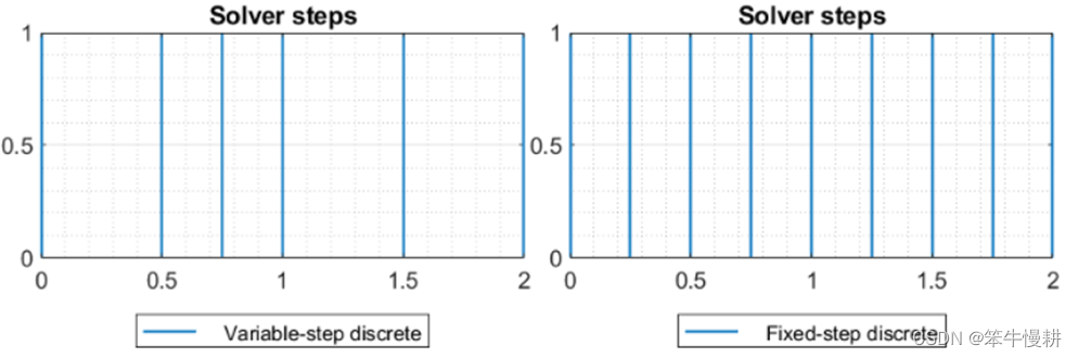
The fixed step solver must take the greatest common divisor of two cycles, i.e 0.25s As its step size , Only in this way can it ensure that it will not miss any effective sampling time of the two signals . The variable step size solver only needs to calculate at the union time of the set of multiples of two cycles , In this way, the number of times it needs to be calculated will be less than that of the fixed step solver .

5.2 Variable step size continuous solver

The variable step size solver dynamically adjusts the step size in the simulation process , On the premise of satisfying the specified error tolerance, the step size should be as large as possible to reduce the computational load and simulation time .

chart 3 Variable step size continuous solver

The use selection decision tree of variable step size continuous solver is shown in the figure above . The variable step size solver can be further divided into one-step or multistep, single-order or variable-order, and explicit or implicit. For more information, please refer to One-Step Versus Multistep Continuous Solvers.

5.2.1 Explicit variable step size continuous solver

Simulink The following are provided 4 An explicit variable step size continuous solver ： ode45; ode23; ode113; odeN. Their similarities and differences are shown in the following table ：

ode45 Based on explicit Runge—Kutta(4,5) The formula ,Dormand—Prince Yes ． It is — A one-step solver (solver). That is to say, it is calculating y(tn) when , Just use the results of the previous step y(tn-1)． For most problems ． In the first simulation 、 You can use ode45 Have a try ．
ode23 Is based on explicit Runge—Kutta(2,3)．Bogackt and Shampine Yes ． For systems with wide error tolerance and slight rigidity 、 It is better than ode45 More effective ．ode23 It is also a one-step solver ．
odell3 It's a variable order Adams-Bashforth—Moulton PECE solver ． When the error tolerance is strict , It is better than ode45 More effective ．odell3 Is a multistep solver , In order to calculate the current result y(tn）, Not only to know the results of the previous step y(tn-1), Also know the results of the previous steps y(tn-2),y(tn-3),…;

【 Suggest 】

When the simulation speed needs to be given priority, you can choose odeN, for instance ：

The dynamic behavior of the model contains a large number of zero crossing sums / Or solver reset
SolverProfiler The analysis of the model did not find any failed simulation step attempts

5.2.2 Implicit variable step size continuous solver

When the simulation problem is rigid , Try the following implicit variable step size continuous solver ：ode15s; ode23s; ode23t; ode23tb. Their similarities and differences are shown in the following table ：

odel5s It is based on numerical differential formulas (NDFs) Variable order solver for ． It is related to the backward differential formula BDFs( Also called Gear Method ) There's a connection ． But more effective than it ．ode15s Is a multistep solver , If you think a problem is rigid , Or in use ode45s When the simulation fails or is not effective enough , You can try odel5s. odel5s It is based on one to five orders NDF Solver for formulas ． Although the higher the order of the formula, the more accurate the result , But the stability will be worse ． If the model is rigid , And it requires good stability , The maximum order should be reduced to 2． choice odel5s When the solver , This parameter will be displayed in the dialog box ． It can be used ode23 Solver instead .odel5s,ode23 Is a constant step size 、 Lower order solver ．
ode23s It's based on a 2 Order improved Rosenbrock The formula ． Because it is a one-step solver , So for the wide error tolerance , It is better than odel5s More effective ． For some use odel5s Not very effective rigidity problem , It can be used to solve ．
ode23t It's using “ free ” Interpolating trapezoidal rule ． If the problem is moderate rigidity , And you need results without digital damping , This solver can be used ．
ode23tb It's using TR-BDF2 To achieve , That is, based on implicit Runge—Kutta The formula , The first stage is trapezoidal regular step size and the second stage is second-order inverse differential formula ． The two levels of computation use the same iteration matrix ． And ode23s be similar , For wide error tolerance , It is better than odel5s More effective ．

5.3 Error tolerance of variable step size solver （Error Tolerances）

5.3.1 Local error Local Error

The variable step size solver uses standard error control techniques to monitor the local error of each simulation time step . At each simulation time step （time step） The solver calculates the state values at the end of the time step and estimates the local errors （local error）. Compare this local error with the acceptable error tolerance （ Including relative error tolerance rtol And absolute error tolerance atol. If the local error of any state exceeds the acceptable error , The solver will reduce the step size and try again .

Relative error tolerance Relative tolerance Represents the ratio of the local error to the state value itself （ The absolute value ） Threshold of . The default threshold is 1e-3, It means that the local error shall not exceed the state value itself 0.1%.

Absolute error tolerance Absolute tolerance , As the name suggests, it is the pointer error （ The absolute value ） Its own threshold , In fact, it means that the current state value is close to 0 The maximum allowable error value when .

Solver requires state i The error of meets the following conditions ：

gif.latex?e_i%20%5Cleq%20max%28rtol%20%5Ctimes%20%7Cx_i%7C%2Catol_i%29

The following figure shows an example of acceptable error determined by relative error tolerance and absolute error tolerance in different intervals ：

chart 4 Relative error tolerance and absolute error tolerance

5.3.2 Absolute error tolerance Absolute Tolerances

In the configuration parameters dialog box of the model （Solver pane of the Configuration Parameters dialog box） Global absolute error tolerance can be set in . This error tolerance applies to all States , It can be set to auto Or a scalar value . If set to auto（ The default value ） Words ,Simulink First, an absolute error tolerance will be set for each state according to the relative error tolerance , If the relative error tolerance reltol Greater than or equal to 1e-3, abstol Will be initialized to 1e-6; If reltol < 1e-3, abstol It will be initialized to reltol * 1e-3. As simulation time goes on , The absolute error tolerance of each state is updated to the maximum value of the state so far multiplied by the relative error tolerance of the state . therefore , If a status value changes from 0 Change to 1, and reltol=1e-3,abstol Is initialized to 1e-6, Then update to... At the end of the simulation 1e-3. If a status value changes from 0 Change to 1000 Words ,abstol By the end of the simulation, it will be updated to 1.

If the absolute error tolerance determined according to the above rules is not appropriate , Users can determine an appropriate value by themselves . for instance , Determine the appropriate value by simulating trial and error . Users can also set AutoScaleAbsTol An adaptive adjustment process that enables absolute error tolerance , For details, see Auto scale absolute tolerance.

There are several modules that allow the user to specify absolute error tolerance for solving state values , As shown below ：

The absolute error tolerance specified for these modules covers the above in Configuration Parameters dialog box Global settings made in . In some cases , Users may want to override global settings , for instance , Because the change range of all module States is very different , As a result, the global setting fails to provide sufficient error control

The absolute error tolerance of the module has the following setting options :

auto
-1(same as auto)
positive scalar
real vector (having a dimension equal to the number of corresponding continuous states in the block)

5.3.3 Tips:

If you choose to set the absolute error tolerance , Please note that , Setting too small will cause the solver to need excessive simulation steps when the state value is close to zero , This causes the simulation to slow down . On the other hand , If the setting is too large , When one or more states approach zero , Simulation results may become inaccurate . See the above figure for the reasons 3.

Once the simulation is over , You can verify the accuracy of your simulation results . The specific way is , Set the absolute error tolerance to a smaller value to re simulate , If the difference between the results of the two simulations is small enough , It shows that the simulation results are accurate enough , This means that the absolute error tolerance is reasonable .

6. A simple example ： Influence of solver selection on simulation results

Consider a simple simulink Model , Because the function of each module is obvious , There's not much to explain here .

There is no discrete sampling module in this model , The default configuration of the solver is shown in the following figure ：

The simulation results are shown in the figure below , Obviously , The curve of simulation output result is not smooth enough , Continuity is not good enough . This is because the default configuration , The number of steps used is 50, That is, the step size is 1. For a simple model like this , Even such a rough configuration , The simulation error is also within the error tolerance （ As a matter of the fact, nothing has been done , At the simulated sampling time , The error is always 0）.