当前位置:网站首页>小样本故障诊断 - 注意力机制代码 - BiGRU代码解析实现
小样本故障诊断 - 注意力机制代码 - BiGRU代码解析实现
2022-06-24 06:57:00 【故障诊断与python学习】
文章目录
1 参考论文
Fault diagnosis for small samples based on attention mechanism
2 开源代码
https://github.com/liguge/Fault-diagnosis-for-small-samples-based-on-attention-mechanism
3.摘要
针对深度学习在故障诊断中的应用,机械旋转设备部件在复杂的工作环境下容易发生故障,工业大数据存在标记样本有限、工作条件不同、噪声等问题。针对上述问题,提出了一种基于双路径卷积与注意机制(DCA)和双向门控循环单元(DCA- bigru)的小样本故障诊断方法,该方法的性能可以通过最新的正则化训练策略进行有效挖掘。利用BiGRU实现时空特征融合,利用DCA提取融合了注意权的振动信号特征。此外,还将全局平均池化(GAP)应用于降维和故障诊断。实验表明,DCA-BiGRU具有出色的泛化能力和鲁棒性,能够有效地进行各种复杂情况下的诊断。
4.故障诊断流程图

5.网络模型
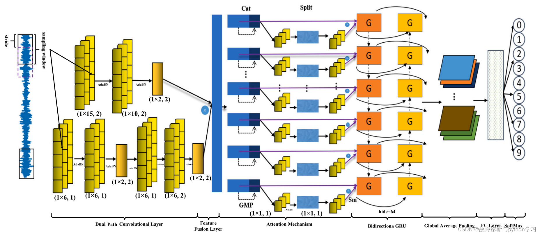
6.网络结构简介
输入1维数据:[batch_size, 1, 1024]–>双通道卷积–>特征融合(cat)–>注意力机制–>Bidirection GRU–>全局平均池化(Global average pool)–>全连接层–>softmax求分类概率
7.网络模型代码
建议使用pytorch,jupyter notebook
7.1MetaAconC
模块代码
import torch
from torch import nn
class AconC(nn.Module):
    r""" ACON activation (activate or not). # AconC: (p1*x-p2*x) * sigmoid(beta*(p1*x-p2*x)) + p2*x, beta is a learnable parameter # according to "Activate or Not: Learning Customized Activation" <https://arxiv.org/pdf/2009.04759.pdf>. """

    def __init__(self, width):
        super().__init__()
        self.p1 = nn.Parameter(torch.randn(1, width, 1))
        self.p2 = nn.Parameter(torch.randn(1, width, 1))
        self.beta = nn.Parameter(torch.ones(1, width, 1))
    def forward(self, x):
        return (self.p1 * x - self.p2 * x) * torch.sigmoid(self.beta * (self.p1 * x - self.p2 * x)) + self.p2 * x


class MetaAconC(nn.Module):
    r""" ACON activation (activate or not). # MetaAconC: (p1*x-p2*x) * sigmoid(beta*(p1*x-p2*x)) + p2*x, beta is generated by a small network # according to "Activate or Not: Learning Customized Activation" <https://arxiv.org/pdf/2009.04759.pdf>. """

    def __init__(self, width, r=16):
        super().__init__()
        self.fc1 = nn.Conv1d(width, max(r, width // r), kernel_size=1, stride=1, bias=True)
        self.bn1 = nn.BatchNorm1d(max(r, width // r), track_running_stats=True)
        self.fc2 = nn.Conv1d(max(r, width // r), width, kernel_size=1, stride=1, bias=True)
        self.bn2 = nn.BatchNorm1d(width, track_running_stats=True)
        self.p1 = nn.Parameter(torch.randn(1, width, 1))
        self.p2 = nn.Parameter(torch.randn(1, width, 1))

    def forward(self, x):
        beta = torch.sigmoid(self.bn2(self.fc2(self.bn1(self.fc1(x.mean(dim=2, keepdims=True))))))
        return (self.p1 * x - self.p2 * x) * torch.sigmoid(beta * (self.p1 * x - self.p2 * x)) + self.p2 * x
代码测试
x = torch.randn(16, 64, 1024)  #假设输入x:batch_size=16, channel=64, length=1024
Meta = MetaAconC(64)  #创建对象时需输入参数width,其为输入数据的channel
y = Meta(x)
print(y.shape)
>>>output
x.shape: torch.Size([16, 64, 1024])
y.shape: torch.Size([16, 64, 1024])
由结果可见,输入x的shape与输出y的shape是相同的
7.2注意力机制
注意力机制结构图

模块代码
class CoordAtt(nn.Module):
    def __init__(self, inp, oup, reduction=32):
        super(CoordAtt, self).__init__()
        # self.pool_w = nn.AdaptiveAvgPool1d(1)
        self.pool_w = nn.AdaptiveMaxPool1d(1)
        mip = max(6, inp // reduction)
        self.conv1 = nn.Conv1d(inp, mip, kernel_size=1, stride=1, padding=0)
        self.bn1 = nn.BatchNorm1d(mip, track_running_stats=False)
        self.act = MetaAconC(mip)
        self.conv_w = nn.Conv1d(mip, oup, kernel_size=1, stride=1, padding=0)

    def forward(self, x):
        identity = x
        n, c, w = x.size()
        x_w = self.pool_w(x)
        y = torch.cat([identity, x_w], dim=2)
        y = self.conv1(y)
        y = self.bn1(y)
        y = self.act(y)
        x_ww, x_c = torch.split(y, [w, 1], dim=2)
        a_w = self.conv_w(x_ww)
        a_w = a_w.sigmoid()
        out = identity * a_w
        return out
模块代码测试
x = torch.randn(16, 64, 1024)  #假设输入x:batch_size=16, channel=64, length=1024
Att = CoordAtt(inp=64, oup=64)  #创建注意力机制对象,输入参数inp和oup参数分别为channel
y = Att(x)
print('y.shape:',y.shape)
>>>output
y.shape: torch.Size([16, 64, 1024])
由结果可见,输入x的shape与输出y的shape是相同的
7.3 BiGRU测试
BiGRU结构图

x = torch.randn(16, 64, 128)  #假设输入x:batch_size=16, channel=64, length=128
gru = nn.GRU(128, 64, bidirectional=True)  #创建GRU对象,128是输入数据x的长度;
                                           #如果bidirectional为False,64是输出数据的长度;如果bidirectional为True,则输出长度为64*2
y = gru(x)
print('y的值:\n',y)
print('y[0]的shape',y[0].shape)
>>>output
y的值:
 (tensor([[[-0.7509, -0.0468,  0.2881,  ..., -0.6559,  0.5780,  0.3481],
         [ 0.4099,  0.1912, -0.2534,  ..., -0.2067, -0.1099, -0.3594],
         [ 0.0275,  0.0937, -0.4309,  ..., -0.6266,  0.5375,  0.2510],
         ...,
         [-0.1896, -0.0118, -0.4895,  ...,  0.2022,  0.3144,  0.1806],
         [-0.5026,  0.4926, -0.2578,  ..., -0.3386, -0.3908, -0.1203],
         [-0.0431, -0.1084,  0.4494,  ...,  0.4320, -0.2916,  0.4126]]],
       grad_fn=<StackBackward0>))
y[0]的shape torch.Size([16, 64, 128])
由结果可以看出,y的输出为一个tuple元组类型,因此使用了y[0]获取里面的tensor数据。
7.4 全局平均池化GAP测试
# 第一步输入x
x = torch.randn(16, 64, 32) #假设输入x:batch_size=16, channel=64, length=128
print('x的值:\n',x)
print('x[0][0]的值:',x[0][0])
print('x[0][0]的平均值:',torch.mean(x[0][0]))

# 第二步进行自适应平均池化
adavp = nn.AdaptiveAvgPool1d(1) #
y = adavp(x)
print('y的值:',y)
print('y的shape:',y.shape)

# 第三步
z = y.squeeze()
print('z的shape:',z.shape)
x的值:
 tensor([[[ 7.8979e-01,  1.3657e-01, -9.9066e-01,  ...,  9.5261e-01,
           9.8295e-02,  6.5511e-01],
         [-3.5707e-01, -2.3277e+00, -3.2558e-01,  ..., -2.2010e-01,
          -1.6210e+00, -1.2564e+00],
         [ 1.0400e+00, -1.8403e-01,  1.1634e+00,  ...,  5.7404e-02,
          -7.0334e-01, -1.5286e-01],
         ...,
         [-1.7541e+00,  5.9410e-01, -1.3539e-01,  ...,  8.6600e-02,
           1.2851e+00, -2.1541e+00],
         [ 1.6649e+00, -3.0008e+00, -6.5557e-01,  ...,  3.8984e-01,
          -2.4122e+00,  1.3892e+00],
         [ 3.2660e-01,  1.4245e+00,  8.2627e-01,  ..., -1.1504e+00,
           8.5084e-01, -2.3794e-02]]])
x[0][0]的值: tensor([ 0.7898,  0.1366, -0.9907, -0.9970,  1.6666, -1.5021,  0.9952,  0.5044,
         0.0828,  1.1746, -1.1589, -1.2519, -1.6039, -0.9943,  0.4700, -0.5370,
         0.5983, -0.6333, -1.3765, -0.9212, -0.3939, -0.7217,  0.4318,  0.4706,
         0.6322, -0.4217, -1.0003,  1.6015,  0.5162,  0.9526,  0.0983,  0.6551])
x[0][0]的平均值: tensor(-0.0852)
y的值: tensor([[[-0.0852],
         [-0.6024],
         [-0.0316],
         ...,
         [ 0.0157],
         [-0.2135],
         [ 0.1926]]])
y的shape: torch.Size([16, 64, 1])
z的shape: torch.Size([16, 64])
由结果可以看出,输入数据x1.shape=[16, 64, 32]全局平均池化是将输入数据的最后一维,及32个数据点取平均值。得到[16, 64]
7.5 整体网络测试
整体网络代码
class Net(nn.Module):
    def __init__(self):
        super(Net, self).__init__()
        self.p1_1 = nn.Sequential(nn.Conv1d(in_channels=1, out_channels=50, kernel_size=18, stride=2),
                                  nn.BatchNorm1d(50, track_running_stats=False),
                                  MetaAconC(50))
        self.p1_2 = nn.Sequential(nn.Conv1d(50, 30, kernel_size=10, stride=2),
                                  nn.BatchNorm1d(30, track_running_stats=False),
                                  MetaAconC(30))
        self.p1_3 = nn.MaxPool1d(2, 2)
        self.p2_1 = nn.Sequential(nn.Conv1d(1, 50, kernel_size=6, stride=1),
                                  nn.BatchNorm1d(50, track_running_stats=False),
                                  MetaAconC(50))
        self.p2_2 = nn.Sequential(nn.Conv1d(50, 40, kernel_size=6, stride=1),
                                  nn.BatchNorm1d(40, track_running_stats=False),
                                  MetaAconC(40))
        self.p2_3 = nn.MaxPool1d(2, 2)
        self.p2_4 = nn.Sequential(nn.Conv1d(40, 30, kernel_size=6, stride=1), nn.BatchNorm1d(30, track_running_stats=False),MetaAconC(30))
        self.p3_0 = CoordAtt(30, 30)
        self.p2_5 = nn.Sequential(nn.Conv1d(30, 30, kernel_size=6, stride=2),
                                  nn.BatchNorm1d(30, track_running_stats=False),
                                  MetaAconC(30))
        self.p2_6 = nn.MaxPool1d(2, 2)

        self.p3_1 = nn.Sequential(nn.GRU(124, 64, bidirectional=True))  #
        # self.p3_2 = nn.Sequential(nn.LSTM(128, 512))
        self.p3_3 = nn.Sequential(nn.AdaptiveAvgPool1d(1))  #GAP
        self.p4 = nn.Sequential(nn.Linear(30, 10))

    def forward(self, x):
        p1 = self.p1_3(self.p1_2(self.p1_1(x)))
        print('p1.shape:',p1.shape)

        p2 = self.p2_6(self.p2_5(self.p2_4(self.p2_3(self.p2_2(self.p2_1(x))))))
        print('p2.shape:',p2.shape)

        encode = torch.mul(p1, p2)
        print('encode.shape:',encode.shape)

        # p3 = self.p3_2(self.p3_1(encode))
        p3_0 = self.p3_0(encode).permute(1, 0, 2)
        print('p3_0.shape:',p3_0.shape)

        p3_2, _ = self.p3_1(p3_0)
        print('p3_2.shape:',p3_2.shape)

        # p3_2, _ = self.p3_2(p3_1)
        p3_11 = p3_2.permute(1, 0, 2)  #
        print('p3_11.shape:',p3_11.shape)

        p3_12 = self.p3_3(p3_11).squeeze()
        print('p3_12.shape:',p3_12.shape)
        # p3_11 = h1.permute(1,0,2)
        # p3 = self.p3(encode)
        # p3 = p3.squeeze()
        # p4 = self.p4(p3_11) # LSTM(seq_len, batch, input_size)
        # p4 = self.p4(encode)
        p4 = self.p4(p3_12)
        print('p4.shape:',p4.shape)
        return p4
代码测试
model = Net()
x = torch.randn(16, 1, 1024) #假设输入x:batch_size=16, channel=1, length=1024
y = model(x)
>>>output
p1.shape: torch.Size([16, 30, 124])
p2.shape: torch.Size([16, 30, 124])
encode.shape: torch.Size([16, 30, 124])
p3_0.shape: torch.Size([30, 16, 124])
p3_2.shape: torch.Size([30, 16, 128])
p3_11.shape: torch.Size([16, 30, 128])
p3_12.shape: torch.Size([16, 30])
p4.shape: torch.Size([16, 10])
8 实验设置
8.1 模型参数设置

8.2 实验数据设置

9 实验验证
案例1:CWRU
不同batch_size下的结果

不同负载下的结果

(后续继续完善)
注:
① 若本论文对你有帮助启发,建议引用本论文~
② 欢迎关注公众号《故障诊断与Python学习》
③ 若有好的开源代码,欢迎后台联系推荐~
边栏推荐
- Model effect optimization, try a variety of cross validation methods (system operation)
- 宝塔面板安装php7.2安装phalcon3.3.2
- Opening chapter of online document technology - rich text editor
- Vulnhub target: boredhackerblog: social network
- 对于flex:1的详细解释,flex:1
- Teach you how to use the reflect package to parse the structure of go - step 1: parameter type check
- JS implementation to check whether an array object contains values from another array object
- Dart development server, do I have a fever?
- Selenium IDE的安装以及使用
- [data update] Xunwei comprehensively upgraded NPU development data based on 3568 development board
猜你喜欢
Simple summary of lighting usage

Swift 基础 Swift才有的特性

Latest news of awtk: new usage of grid control

Introduction to software engineering - Chapter 2 - feasibility study
![[C language] system date & time](/img/de/faf397732bfa4920a8ed68df5dbc48.png)
[C language] system date & time

How to cancel the display of the return button at the uniapp uni app H5 end the autobackbutton does not take effect

Gossip: what happened to 3aC?

Écouter le réseau d'extension SWIFT (source)
Swift foundation features unique to swift

Ad-gcl:advantageous graph augmentation to improve graph contractual learning
随机推荐
The monthly salary of two years after graduation is 36K. It's not difficult to say
1279_ Vsock installation failure resolution when VMware player installs VMware Tools
[008] filter the table data row by row, jump out of the for cycle and skip this cycle VBA
Swift foundation features unique to swift
SVN实测常用操作-记录操作大全
Swift extension chainlayout (UI chain layout) (source code)
Gossip: what happened to 3aC?
QOpenGL显示点云文件
Analysis of abnormal problems in domain name resolution in kubernetes
Live wire, neutral wire and ground wire. Do you know the function of these three wires?
Swift 基础 闭包/Block的使用(源码)
2021-03-04 COMP9021第六节课笔记
GraphMAE----論文快速閱讀
[测试开发]初识软件测试
Search and recommend those things
[test development] first knowledge of software testing
软件工程导论——第三章——需求分析
transformers PreTrainedTokenizer类
Graphmae - - lecture rapide des documents
JVM underlying principle analysis