[theory] deep learning in the covid-19 epic: a deep model for urban traffic revitalization index

Deep learning in the COVID-19 epidemic: A deep model for urban traffic revitalization index

original text , see here
author ：Zhiqiang Lv , Jianbo Li , Chuanhao Dong , Haoran Li , Zhihao Xu
Periodical ： Eiswell Data & Knowledge Engineering,2021
keyword ：COVID-19; Traffic revitalization index ; data mining ; Data model ; Mining methods and algorithms

Abstract

The study of traffic revitalization index can be used for urban management 、 Epidemic prevention and control 、 Provide support for the formulation and adjustment of relevant policies such as returning to work and production . This paper proposes Depth prediction model of urban traffic revitalization index a deep model for the prediction of urban Traffic
Revitalization Index(DeepTRI).DeepTRI The data of COVID-19 in major cities in China and the traffic revitalization index model are constructed .29 The location information of cities constitutes the topological structure of the graph . The spatial convolution layer proposed in this paper captures the spatial correlation features of graph structure . Special Graph Data Fusion The module distributes and fuses the two types of data according to different proportions , Increase the spatial correlation trend of data . In order to reduce the complexity of the computing process , The time convolution layer replaces the gating recursion mechanism of the traditional recurrent neural network with the multilevel residual structure . The dynamic change of the receiving field is controlled by the expanded convolution whose expansion factor varies with the convex function , Use causal convolution to fully mine the historical information of data , Optimize long-term forecasting capability . By comparing with three baselines ( Traditional recurrent neural networks 、 General spatiotemporal model and graphical spatiotemporal model ) A comparative experiment of , Shows DeepTRI Advantages in evaluation indicators , And solved Edge value under fitting and local peak under fitting Two major under fitting problems .

1. Introduction

1.1. Urban traffic revitalization index

The traffic condition reflects the operation of the city 、 Important characteristics of health and order in production and life . Road conditions and travel data [1] It can well reflect the recovery of urban production and consumption activities . City Traffic revitalization index traffic revitalization index ( This paper is abbreviated to TRI ) The data is provided by didi platform [2] Calculation . Researchers of didi platform fit urban traffic trajectory and road congestion data 、 Cross validation and weighting .TRI It is an important indicator to reflect the urban traffic conditions .TRI Based on Intelligent Transportation Technology and data analysis capability , Let users visually see the recovery of traffic in each city . It provides more information for orderly promoting the recovery of production and life . It's scientific 、 It objectively reflects the urban traffic activities . Overall speaking , Flow activity varies with TRI To increase by .TRI It's specifically for 2019 The indicators set up for the impact of coronavirus disease on urban traffic . stay TRI The concept of ,2019 At the end of the year, cities during the non epidemic period TRI near 1. With 2019 The outbreak of COVID-19 at the end of the year , Transportation is greatly affected , This directly leads to the TRI Drop sharply . Facing the epidemic situation , The government and health departments have formulated and implemented various epidemic prevention measures . Production and living in various cities are gradually restored . The vitality of urban traffic will gradually return to the normal level .

Transportation industry is the basic and leading industry of the national economy , It is an important part of the national economy . The development of transportation industry has promoted the rapid economic growth . In turn, economic growth has driven the development of transportation industry . therefore ,TRI It has dynamic synchronization with economic development . surface 1 Shows the city GDP And TRI The relationship between . China's GDP It is calculated on a quarterly basis , So we calculated 2020 In the first two quarters of the year, the number of GDP And the average TRI. It can be seen from the statistics that , Almost all the cities experienced in the second quarter GDP A huge increase in . meanwhile ,TRI It also increases . Due to the outbreak of the second epidemic , Xiamen second quarter GDP It's down . In the second quarter TRI Declined 0.4219%. It can be seen from the above results , No matter what GDP Increase or decrease ,GDP And TRI Are dynamically synchronized .

1.2. The economic impact of the COVID-19

The COVID-19 has had a profound and significant impact on the transportation industry [3-6], It has had a serious impact on the world economy [7-9]. With the spread of the epidemic , Industrial demand is declining , Increased risk of viral infection , China's transportation services have dropped dramatically .2019 end of the year , Under normal circumstances , Chinese cities TRI near 1. But because of the spread of the epidemic ,2020 At the beginning of the year, all cities in China TRI There have been different degrees of decline . chart 1 Shows 2020 The relationship between the year-on-year growth of China's industrial added value at the beginning of the year and the number of suspected cases . We can know ,2 The number of suspected cases reached a peak in January . Affected by the epidemic ,3 Industrial added value fell sharply in January , Even negative growth .3 Since the month , With the help of strong prevention and control measures , The domestic epidemic has gradually subsided , Suspected cases have decreased rapidly . Urban production and living are gradually restored , The traffic vitality gradually recovers to the normal level [10].

Fig.1 The relationship between the year-on-year growth of industrial added value and the number of suspected cases . The abscissa represents the date . The industrial added value is in direct proportion to the year-on-year growth , Corresponds to the spindle on the left . The unit of suspected cases is 1 ten thousand ( people ), Corresponding to the second axis on the right .

1.3. Graph neural network

With the development of deep learning , Images 、 Major technological breakthroughs have been made in the fields of speech and naturallanguageprocessing [11-13]. Deep learning is good at handling structured data , Such as voice 、 Images and text . However , There are a lot of unstructured data in the real world , Such as social network topology 、 Knowledge map, etc . Unstructured data does not have the same spatial location as images , The data range is arbitrary , And the topology is complex . Figure neural network [14] And the most basic structure of neural network (Multi-Layer Perception, MLP) comparison , An adjacency matrix is added to participate in the process of matrix calculation , Such as type (1) Shown .$\sigma$ Represents nonlinear transformation .$A$ Denotes the adjacency matrix .$X$ Represents the characteristic matrix ,$W$ Represent the weight matrix .
$$H=\sigma (AXW)\text{\hspace{1em}(1)}$$
chart [15] Spatiotemporal network The spatial correlation and time dependence of data are captured . Spatiotemporal graph has global graph structure , The value of each node changes over time . for example , Many works have established PeMS data[16] Space-time network . The basic implementation process of these networks takes the data station of the power module as the node of the graph . The input of nodes is time series , Such as traffic flow 、 The speed of the car 、 Road occupancy . The edge of the spatiotemporal network graph represents the longitude and latitude distance between data stations . The task of graph spatiotemporal network is to predict the future value of nodes or the type of nodes . The spatial correlation between cities conforms to the topological relationship . This topological relation can be transformed into adjacency matrix [17], It is used in the calculation of graph neural network , Such as chart 2 Shown .

Fig.2 The process of transforming urban spatial correlation into adjacency matrix . The points on the map on the left represent the locations of some cities in China . The graph in the middle shows the topological relationship of the city location . The right figure shows the adjacency matrix corresponding to the topological relationship of the city location .

1.4. Contribution

Based on the above research theory , In this paper, the spatial location relationship of Chinese cities is transformed into a graph structure , Combined with the data of COVID-19 and TRI data , Complete the task of urban traffic recovery prediction . The main contributions of this paper are as follows :

• This paper presents a new kind of Picture time and space network (Deep Model for Traffic Revitalization index ,DeepTRI). This is the first one used to predict TRI Space time network , And the first one to TRI And COVID-19 The work of combining epidemic data .
• According to the characteristics of epidemic data , A special Graphics data fusion (GDF) modular .GDF Different weights are given to the four types of epidemic data . By convoluting the network with a graph (GCN) and GDF Composed of a spatial convolution layer , Fully mining the spatial correlation characteristics of graph structure .
• This paper designs a Time convolution , Time series feature used to calculate time correlation . In order to overcome the shortcomings of traditional recurrent neural network which does not support parallel computing and slow training speed . The time convolution layer uses Multilayer residual structure It replaces the gating mechanism of recurrent neural network . We make use of Index is 2 The expansion factor of the convex function of To control the depth of the network Receptive domain , And make use of Causal convolution mechanism To keep the influence of historical data on time characteristics .
• We make use of DeepTRI Yes TRI Data and 4 Class popular data for training , And establish 3 Class baseline ( Traditional recurrent neural networks 、 Graph convolution and graph spatiotemporal network ) To verify DeepTRI Performance of . Experimental results show that ,DeepTRI It has obvious advantages in evaluating indicators and solving the two major under fitting problems of edge value under fitting and local peak under fitting .

2. Related work

Of this work The basic principle yes Using location information between cities and TRI Time series change to build graph structure model . Mapping the basic features between cities to the boundary value information of the graph . Will the city TRI The temporal characteristics of the graph are mapped to the temporal data of the graph nodes . therefore , The knowledge involved in this work is to use adjacency matrix to establish The graph structure And for Unstructured graph Data forecast of .

2.1. Basics

Figure the basic design process of spatiotemporal network is to integrate traffic data ( Vehicle flow 、 The speed of the car 、 Road occupancy rate, etc ) The time variation of is designed as the input value of the graph node , The position relationship between nodes is designed as the weight of graph edges . The traditional methods can not meet the requirements of long-term traffic prediction , There are complex nonlinear problems in traffic data , use Spatiotemporal graph convolution network (Spatial-Temporal Graph Convolutional Networks, STGCN)[18] The time series of traffic data are predicted based on graph neural network . In order to improve the training speed of the model ,STGCN¹ Using pure convolution structure to construct spatiotemporal convolution block . The spatiotemporal convolution block is composed of two temporal gate convolution blocks and a spatial schema convolution block . And statistical methods (ARIMA)、 Traditional machine learning methods are compared with spatiotemporal models ,STGCN It has advantages in accuracy and training speed . Aiming at the problem of traffic flow prediction in traffic network , Put forward Attention based spatiotemporal graph convolution network (ASTGCN)[19].ASTGCN² The three time characteristics of traffic flow ( Recent data 、 Daily cycle data and weekly cycle data ) Build a model . The calculation process of these three time characteristics is independent of each other . Each computing process first uses the time attention mechanism to calculate the dynamic dependencies between different times , The spatial attention mechanism is used to calculate the dynamic correlation between different positions . Last , The space-time convolution module is used to calculate the spatial characteristics of the graph and the dependence of adjacent nodes in the traffic network . take ASTGCN Methods and traditional methods 、 Recursive neural networks and other graphical spatiotemporal networks are compared . Even if there is no attention mechanism ASTGCN The accuracy of the model is also higher than that of other models . After adding the attention mechanism ,ASTGCN stay RMSE The index fell on average 6.2%, stay MAE The index fell on average 4.5%. Regardless of the attention mechanism ASTGCN The accuracy of the model is higher than that of other models . After adding the attention mechanism ,ASTGCN Of RMSE Declined 6.2%,RMSE Declined 4.5%. Time graph convolution network (T-GCN³)[20] Combined graph convolution network (GCN) And gated recursive unit (GRU) To complete the task of speed prediction .GCN By constructing the topological relationship of the traffic network ( Connectivity ) To calculate spatial correlation .GRU The time dependence is calculated by calculating the time series change of vehicle speed .

2.2. Adjacency matrix

STGCN and ASTGCN The adjacency matrix of represents the adjacency matrix between nodes Distance relationship . and T-GCN The adjacency matrix of represents the connectivity between nodes . therefore ,T-GCN The adjacency matrix of is composed of 0 and 1 form . In a comparative experiment , although T-GCN Good performance in long-term forecast , However, the prediction results of edge value and local peak value are not well fitted . Different from the above research , Diffusion convolution recurrent neural network (Diffusion Convolutional Recurrent Neural Network, DCRNN⁴)[21] Using digraph to calculate the spatiotemporal characteristics of traffic data .DCRNN Two way random walk mechanism Calculation Spatial correlation , Using encoders - Decoder mechanism calculation Time relevance .DCRNN The diffusivity of is mainly reflected in the fact that the whole network generates more predictions by maximizing the time range of the target value . Compared with the experimental baseline ,DCRNN Has improved the accuracy of 12% ~ 15%.GCNN-DDGF⁵[22] Four adjacency matrices are designed based on the data of shared bicycle system , Include Spatial distance matrix 、 Demand matrix 、 Average travel duration matrix and demand correlation matrix . It calculates the relationship between different types of sites , To forecast the short-term demand in the large-scale shared bicycle network . With data-driven graph filter (Data-driven Graph Filter, GCNN-DDGF) Graph convolution neural network [23] Pay attention to the similarity of dynamic flow between nodes . Three models of establishing adjacency matrix are proposed , Include Distance map 、 Interaction diagram and Correlation chart . Distance map The distance graph The reciprocal of node distance is used to represent the weight between nodes . Interaction diagram The interaction graph The number of driving records between two nodes is used to represent the weight between nodes . Correlation chart The related graph Use Pearson correlation coefficient (Pearson Correlation Coefficient) Calculate the correlation between the inflow or outflow of two nodes in a fixed time interval , As the weight between nodes .GCNN-DDGF These three adjacency matrices are not calculated separately , It is Three adjacency matrices are fused into one adjacency matrix , And the process of graph convolution .

2.3. Special graph

In the field of taxi demand research , In order to capture the relative relationship of passenger spatial motion between different areas , be based on grid Embedded multi task learning (GEML)[24] Divide the urban area into grids . The graph node represents the geographical area ( Grid form ), The edges between the nodes represent passenger demand .GEML Use multi task learning module to calculate time series data ( The inflow and outflow of the grid ) Dependency characteristics of . Spatiotemporal synchronous graph convolution network (STSGCN)[25] A special graph structure is proposed ( Local spatiotemporal map ). The local spatiotemporal graph mainly focuses on the three effects of nodes on adjacent nodes : Correlation effects based on spatial relationships 、 Based on the time dependence of the same node and the spatiotemporal correlation of adjacent nodes in the process of transferring from the previous time step to the next time step . In the local spatiotemporal graph , Each node not only has the value of its neighbor nodes with the same time step , It also has the values of the two time steps before and after it . The value of the neighbor node in the two time steps before and after it is taken as the second-order neighbor . Local spatiotemporal convolution uses graph convolution to make each node consider its own relationship with its multi-level neighbors . The interaction between each node and its first-order nearest neighbor includes spatial correlation and temporal correlation . The influence between second-order neighborhoods includes temporal and spatial correlation . Work [26] Two methods for graph convolution are proposed Adaptive module : Node adaptive parameter learning node adaptive parameter learning**(NAPL**) And data adaptive graph generation data adaptive graph generation(DAGG).NAPL Parameters are not shared among all nodes , But it maintains a unique spatial parameter for each node , To learn the pattern of a particular node .DAGG It overcomes the shortcoming that the traditional graph convolution network needs to define the adjacency matrix in advance , Implicit interdependencies between nodes can be calculated automatically from the data .

3. Model design

3.1. Overview

DeepTRI Its main structure is as follows chart 3 Shown . Based on the spatial location relationship between cities , Established Graph structure adjacency matrix （$W$）[ chart 3 Left center ]. City TRI data $\{V_t\}$ It is processed in the form of adaptive graph structure , Then participate in the calculation process of the first time convolution layer . First time convolution layer pair TRI Scale compression and feature transformation of data , Instead of simple linearization and splicing .$W$ With the first time convolution layer （$\{T{C}_t^1\}$） Combined with the output of , To calculate TRI Spatial correlation of data . This GDF The cities are integrated and calculated （$\{U\}$） And the whole country （$\{C\}$） Multiscale characteristics of epidemic data . The second time convolution layer calculates the time dependence of the fused data （$\{S{C}_t\}$）. from chart 3 It can be seen that , Time convolution Temporal Convolution Layer from Multistage residual block multi-level residual blocks form . Each remaining block contains Causal convolution and Expansion convolution . Causal convolution Associate the three characteristics of the current node of the hidden layer with all historical information , Thus, the time dependence of the sequence is enhanced . Expansion convolution So that the convolution process of hidden layers can obtain a larger dynamic receptive field without changing the number of hidden layers .DeepTRI It consists entirely of convolution networks , Therefore use BatchNorma2d To prevent gradient disappearance and gradient explosion of convolution network . Last , Fully connected layers Mapping data features to sample space , To get the final output （$\{v{\prime }_t\}$）.

Fig.3 DeepTRL Structure

3.2. Definition

TRI The prediction problem can be defined as the model based on historical data $(\{v_{t-s},\cdots ,v_{t-2},v_{t-1}\})$ For the next time interval $t$ data $(v_i)$ The forecast ,$s$ Represents the number of historical data , As formula (2) Shown .$F$ How to build the representation model .
$$v_t^{\prime }=F([v_{t-s},\cdots ,v_{t-2},v_{t-1}])\text{\hspace{1em}(2)}$$

The topological relationship between cities is in a graph structure $G=(W,V)$ describe .$W$ Denotes the adjacency matrix ,$V$ At what point in time does each city TRI data .

The input data of the model has four dimensions , Namely [batch size, node count, time step, channel]. Batch size Indicates the number of samples selected in a period . Number of nodes Indicates the number of city nodes . Time step Days . passageway Represents the number of data characteristics .

The first time the convolution layer realizes the linear change of the data and the calculation of the underlying characteristics , Its shape is [batch size, node count, time step – k + 1, Output1].$k$ Is to calculate the size of the convolution kernel of the first sequential convolution layer .$output1$ Is the output dimension of the first sequential convolution layer .

Spatial convolution consists of two processes (GCN and GDF).GCN It only changes the data characteristics , Its final shape will not change .GDF The number of cases cured in the country concerned , So the shape increases 1, Its shape is [batch size, node count, time step – k + 1, Output1 + 1].

The second time convolution layer calculates the time dependence of the data features to form high-level features . Its shape is [batch size, node count, time step – 2(k + 1), Output2].$Output2$ Is the output dimension of the second time convolution layer .

The output value of the model is generated by the full connection layer , Its shape is [batch size, node count, time step]. The value of the time step represents what the model needs to predict TRI The scope of the . for example , When the time step is set to 3 when , The model predicts the future of each city in the next three days TRI value .

3.3. Spatial convolution layer

The main function of the spatial convolution layer is to calculate the TRI Spatial correlation with epidemic data . According to the distance between cities , A map consisting of urban distribution is established .GDF Through the multi-scale method GCN The output of is fused with epidemic data . what's more , Global development indicators give different weights to different types of epidemic data .

Graph convolutional network

GCN The basic process of the graph is that each node of the graph is affected by adjacent and further nodes at any time , And change your state , Until it finally reaches equilibrium . The closer the adjacent nodes are , The greater the impact on the original node . Laplacian matrix can make a positive comparison between the transfer intensity of data and the difference of states . In order to add the influence of the original node on itself to the calculation process , Using the improved Laplace matrix , Such as type (3) Shown .

$$L=D^{-1/2}A{D}^{-1/2}\text{\hspace{1em}(3)}$$
$A$ Express $W$ Add adjacency matrix after self ring ,$D$ Express $A$ Degree distribution matrix of . It adds its own degree matrix , The self transfer problem is solved . The normalization operation of adjacency matrix is realized by multiplying both sides of adjacency matrix by the value of square root and inverted node degree . The original spectral convolution realizes the filtering of the product of each node and the Fourier transform . however , Because the eigenvector is a high-order variable , And the decomposition efficiency of Laplacian matrix in large graph structure is low , We use k Chebyshev polynomial of order to approximate the calculation process of Laplace matrix , Such as type (4) Shown .
The formula 4

$y$ Represents the output of the first sequential convolution layer .$T_i(\tilde{L})$ The calculation process of is shown in The formula 5, It represents the recursive definition of Chebyshev polynomials . This method is called K- Local convolution algorithm K-localized convolution algorithm, It ensures that the current node only considers values in K The impact of nodes within the scope . The above process greatly reduces the time complexity of graph convolution network .
The formula 5

Graph data fusion

TRI Data passes through the first time convolution layer , formation TRI The underlying characteristics of the data . after GCN Handle , It preliminarily has the spatial correlation characteristics of urban location . The above process is chart 4 Medium matrix (a) Data processing process .GDF about DeepTRI Is indispensable to , Because it represents inter city TRI A matrix of relationships (a) The spatial characteristics of are not significant . No, GDF Of DeepTRI The experimental results of lead to poor performance , We have proved this theory in experiments .GDF Through a multi-scale approach , Compare the epidemic data of each city with that of each city TRI Data and national epidemic data , Increase the spatial characteristics of urban traffic revitalization . We passed on behalf of TRI And the matrix of basic characteristics of the original epidemic data (a) Conduct concat And weighted summation of different dimensions to achieve multi-scale fusion . The multi-scale fusion process improves the accuracy of prediction by fusing different levels of semantic features .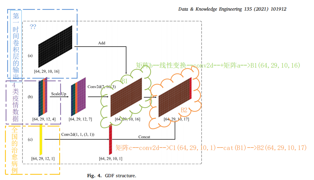

Fig.4 GDF Structure about chart 4 Medium matrix (b) Calculation process ,GDF In the modeling process, the proportion of different types of epidemic data is considered first .DeepTRI There are four types of epidemic data used , Include ** Number of confirmed cases 、 Number of suspected cases 、 Number of cured cases and number of dead cases **.4 Although the data of this kind of epidemic situation are all about COVID-19 Epidemic , But the distribution characteristics are different , Such as chart 5 Shown . chart 5 It shows Chengdu 3 Months TRI and 4 Changes in the data of epidemic like diseases . Changes in cured cases and TRI There is obvious dynamic correlation , The other three items of data are related to TRI There are obvious differences . therefore ,GDF According to the data of four kinds of epidemic situation, it is allocated in proportion TRI Dynamic correlation of .

Such as chart 4 Calculation process , Mapping the four types of epidemic data into a matrix (b) Medium 4 Channels , And will represent the channel for curing cases Linearize to 7 Dimensions . The proportion of the four kinds of data is 1:1:1:4. After the proportional distribution process , Characteristic matrix and longitude Con2d Processed matrix (a) Have the same dimension , The convolution kernel is 3×3. Because at this point the matrix (a) and (b) Have the same matrix dimension , So we apply to these two matrices Weighted summation . The matrix represents the cured cases in the country . After passing with 3×1 Kernel Conv2d after , It has preliminary data characteristics . Last , Compare the matrix with (a) and (b) The result matrix of feature addition Merge , complete GDF Multi-scale data fusion process .

Fig.5 The time curve of the three and four types of epidemic data in Chengdu . The abscissa represents time （ God ）. The vertical coordinate on the left indicates TRI Value . The vertical coordinate on the right indicates the number of people .

Causal convolution

Causal convolution theory Used to track more distant historical information [29], Causal convolution The formula is as follows （6） Shown .$\{x_1,x_2,\cdots ,x_t\}$ It's the input sequence $\{y_1,y_2,\cdots ,y_t\}$ Is the output order of hidden layers , also $\{f_1,f_2.\cdots ,f_k\}$ Is a filter sequence . Causal convolution only focuses on historical information and ignores future information .$y_t$ The results can only be traced back to $x_t$ Previous data . 𝐾 The bigger it is , More traceable historical information . If the original input sequence of the current layer is [0,i], Then the original input sequence of the next layer will become [0,i+1].
The formula 6

Dilated convolution

In deep networks , To increase Receptive domain receptive field, Reduce computation , The model always needs downsampling . Although the accepted domain can be increased , But the spatial resolution is reduced . In order not to lose resolution and still expand the receptive field , We used Expansion convolution [30]. The expansion convolution has a parameter that controls the expansion rate （d）. Convolution kernel is used d-1 Numbers 0 fill . therefore , When setting different expansion rates , The accepted domain will be different . The above process can capture multi-scale information . The expansion convolution formula is as follows: （7） Shown .
The formula 7

𝑑 Represents the expansion factor （ Expansion rate ）, It varies according to the convex function .𝑑 The range of values When the index is 2 Within the scope of . increase 𝑑 or 𝐾 You can increase the range of accepted domains . However , Receptive domain The information obtained by long-distance convolution has no correlation with the deepening of the network layer , This means that local information of the model is lost , Cause local information loss . therefore , We change the expansion factor according to the convex function , Such as chart 6 Shown $d$ The change of . This design pattern ensures that the range of receptive field in the depth network is limited , Reduce the loss of local information . The information transmission of dense neurons makes the model more accurate in the calculation of deep features .

Fig.6 The structure of time convolution

Multi-level residual structure

To reduce the complexity of the training process , In traditional recurrent neural networks , Use Residual structure residual structure Instead of Door structure gating structure, Such as chart 7 Shown . The residual structure mainly includes two-layer convolution network and nonlinear mapping process . Weight criteria 【31】 It's how to use it （ Heavy parameterization and weight standardization ） To achieve data standardization . Weight norm is usually used to accelerate model convergence . By normalizing the weights , The gradient range when the gradient is rotated can be suppressed , Realize the self stabilization of gradient .

We use Tanh As the activation function after convolution network , Here's why ：
The... Used in this experiment TRI The value range of the data is [0,1]. After loading the data , perform Z Score standardization process .Z The scoring formula is as follows .
The formula 8

$X$ Represents raw data ,$\bar{X}$ Means mean ,$s$ Means standard deviation . adopt Z The calculation process of the score , The difference between the original data and the average value is saved . therefore 𝑍 The average of is equal to 0.𝑍 Data greater than the average is positive ,𝑍 Data less than the average is negative .TRI After data standardization , Its minimum value is −2.399, The maximum value is 1.415.Tanh The average value of the function is 0, This is more conducive to improving training efficiency . because Tanh The output range of is [−1,1], The gradient value of the parameter has the opposite sign in the training process , Therefore, it is not easy to see aliasing when updating weights , And it's easy to reach the best value 【32】.

3.5. Post-processing

Based on the above Weight Norm Theory , We added a batch norm to the data normalization process [33], To solve the problem of unstable performance caused by too much data after activating the time convolution layer .BatchNorm As formula （9） Shown .
The formula 9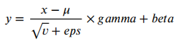

𝜇 and 𝑣 Are the mean and variance of the input data . This 𝑒𝑝𝑠 It is a stability factor added to improve the stability of the calculation process , Its value is equal to 1e-5.gamma and beta Is a coefficient matrix that can be learned . Data normalization process The gradient direction can be lowered to the direction of the vertical contour of the space . The above process can improve the convergence speed of the model , The weight of each level of data can be averaged in the feature calculation , Improve the accuracy of the model . Last , The complete connection layer maps the distributed features of network computing to the sample target space .

4. Experiment

4.1. Data preparation

This experiment uses TRI data [2] The time range is 2020 year 2 month 10 solstice 2020 year 6 month 30 Japan .TRI The time type of data is continuous working days . It includes China 29 Major cities . By fitting the massive traffic data provided by didi travel platform 、 Cross validation 、 Weighted to get TRI data . It can make science 、 Objectively reflect urban traffic activities . The change trend of the index can reflect the trend of traffic activities , So as to indirectly reflect the trend of urban recovery . Epidemic data include 29 Number of confirmed cases in cities 、 Number of suspected cases 、 Number of cured cases 、 Number of deaths 4 Such data and the number of cured cases nationwide . The time range of popular data is similar to TRI Same data . The epidemic data comes from the National Health Commission of China [34].

4.2. Index comparison

Base lines

We set up three types of baselines to verify the performance of the model , Including the traditional recurrent neural network 、 Spatiotemporal neural network and graphical spatiotemporal neural network . All models are trained and evaluated on the same data set . The experimental results are the average of multiple training and evaluation results . The model structure of various baselines in the experiment is as follows :

• LSTM[35]: The data transmission status is controlled through the gating mechanism . With the traditional RNN Just mechanically superimpose a memory ,LSTM Retain long-term memory , Ignoring unimportant information .
• GRU[36]: Its input-output structure is similar to that of the traditional RNN be similar , Deal with logic and LSTM be similar . And LSTM comparison ,GRU A door control is missing inside , Parameters are also better than LSTM Less , But can achieve and LSTM Similar function and precision . Considering the computing power and time cost of the hardware ,GRU It is the choice of more researchers who study deep learning .
• STDN[37]: Use local CNN and LSTM Calculate spatiotemporal information . Part of the door control CNN Modeling spatial dependencies using dynamic similarity between regions . Cycle shifting attention mechanism is used to learn long-term cycle dependence . Last , The attention mechanism is used to model long-term periodic information and time translation .
• GCN[38]: It uses a filter to weighted sum pixels in a certain spatial region , A new feature representation is obtained . The weighting coefficient is the parameter of convolution kernel .
• STSGCN[39]: It consists of multiple graph convolution operations and an aggregation operation . The output of each graph convolution operation will be added to the input of the aggregation layer in a way similar to the residual neural network . Use the largest pool to achieve aggregation .
• GCNN-DDGF[21]: Traditional convolution network and graph convolution network based on data-driven filtering are used to capture spatial correlation . It USES LSTM Structure to capture the time dependence of data characteristics .
• DCRNN[21]: In the design of adjacency matrix , Using digraph to calculate the spatiotemporal characteristics of data . We use its two-way random walk mechanism to calculate the spatial correlation between cities , And use the encoder - Decoder mechanism to calculate the time dependence of data
• GEML[24]: It divides urban areas into grids , But this work is aimed at the TRI Relationship , Therefore, the grid division of a single city is not applicable to this work . We only used GEML The model results , Multi task learning module .
• DAGG[26]: There is no need to define the adjacency matrix representing the urban spatial relationship in advance . During the training , It can automatically establish the interdependencies between urban nodes .
• T-GCN[19]: The model combines graph convolution network (GCN) And gated recursive unit (GRU). adopt GCN Learn complex topology to obtain spatial correlation , adopt GRU Learn the dynamic changes of traffic data to obtain time correlation .
• STGCN[17]: Construct a continuous three-layer convolution network and one-layer convolution network GCN The space-time convolution block (ST-Conv block). The data goes through two layers ST-Conv Block handling .
• ASTGCN[18]: It uses a space-time block composed of a spatial attention layer and a temporal attention layer (ST-BLOCK). The data goes through two layers st - block Handle . Last , It performs a full connection process with three temporal characteristics .

Index introduction

Root mean square error is used in this experiment (RMSE)、 Mean absolute error (MAE) And mean absolute percentage error (MAPE) Three indicators to evaluate the performance of the model , Such as the type (10) Shown .
The formula 10

MAE and MAPE It can measure the accuracy of the prediction results of the model , But they are all based on the calculation process of absolute error . Although the absolute error can get an evaluation value , However, we cannot know the performance of the model represented by this evaluation value . Only through the comparison between models , Only then can we know the best model . therefore , The evaluation process of this experiment also uses RMSE.RMSE It is used to measure the deviation between the predicted value and the real value . It is very sensitive to very large or small errors in a set of data . therefore ,RMSE Can well reflect [40] Accuracy of prediction results .

The evaluation results of each model on the three indicators are as follows surface 2 Shown .GRU and LSTM It is a traditional recurrent neural network , The worst performance . Because they can't handle complex spatial relationships .STDN and GEML Based on the traditional recurrent neural network model, a convolution network is added to calculate the spatial relationship , The accuracy of the model is improved . But it is not a graph structure model , There was no significant effect in this experiment .GCN Suitable for calculating the spatial relationship of graph structure , But it lacks the ability to rely on computing time characteristics , So the performance is not optimal . The city information and TRI Data features are very obvious and rich . And automatic DAGG Figure structure model comparison , The adjacency matrix directly established in this work is more effective . Figure spatiotemporal neural network (GCNN-DDGF, DCRNN, STSGCN, T-GCN, ASTGCN and STGCN) The basic process is to use GCN To calculate spatial relationships , Using recurrent neural network to calculate time correlation . therefore , In the process of recursive modeling, it is impossible to obtain the deep multi-scale context features of data .

Compared with the above figure neural network ,DeepTRI It has a significant impact on the three dimensions of time , Minimum error . This is because DeepTRI Considering the epidemic data TRI The temporal and spatial effects of change . And STGCN Compared with the three-dimensional time index , The error reduction rate is as follows: surface 3 Shown . When DeepTRI The time step is 2d when , Maximum reduction ratio . This is because DeepTRI The causal convolution mechanism of time convolution layer can retain all historical information , More suitable for long-term information calculation .

4.3. The effect of GDF

GDF It plays an important role in the training process of the model .GDF The impact is shown in the figure 8 Shown . chart 8 For two models 100 individual epoch Change in loss value , The experimental parameters are exactly the same . In the early stages of the training process , No, GDF Of DeepTRI Convergence is very slow . Even if the medium-term losses are significantly reduced , But the end result is not ideal . stay GDF With the help of the ,DeepTRI It can converge quickly , And keep the training loss in a small range , Without over fitting . This is because the epidemic data and TRI It has obvious dynamic correlation , and GDF It enlarges the dynamic correlation between the two . Last ,GDF The weighted feature of the model to the modeling target is enhanced .

Fig.8 GDF The role of . The abscissa represents time ( God ). The ordinate represents the value of the loss .

4.4. Spatial-temporal results

This chapter mainly focuses on two under fitting problems in the comparison of actual results of the model , Including edge value under fitting and local peak [41] Under fitting .

Under-fitting of edge values

Fig.9

The problem of edge value under fitting This means that the model is correct for TRI The prediction result of median value is better , But for smaller or larger TRI The prediction result of is poor . Such problems as chart 9(a)、(b)、( c) Shown , for example (a) in TRI The predicted value of is in the interval [48,78] Is basically consistent with the real value , And in the interval [38,48]、[78,88] There is an under fitting problem in the predicted value . The prediction results are approximate to a straight line . The problem of boundary value under fitting is reflected in all city matrices . chart 10(a) and (b) Represents the space width of the edge value . The reason for this problem is that the intermediate values in the data set overlap , The features are obvious , The edge data is sparse , Insufficient spatial correlation between edge values .

Fig.10 Of all nodes in a single time period TRI value . The abscissa represents time ( God ). The ordinate represents TRI Value .

Fig.11 Single node TRI Over time . The abscissa represents time ( God ). The ordinate represents TRI Value .

Figure neural network can effectively avoid the above problems , Such as chart 11(a) Shown .(a) Is based on GCN Of TRI Modeling results , It effectively avoids the problem of edge value under fitting .GCN Able to capture the spatial relationship of graph structure , Make the predicted value have the fitting ability to the data of all intervals . chart 11(b) and ( c) It shows the results of complex graph spatiotemporal network . From their comparison results, we can see that , be based on GCN The spatiotemporal network can further suppress the under fitting problem of edge values . Specially ,T-GCN As a graph spatiotemporal network , It shows a certain degree of boundary value under fitting problem . This is because T-GCN Use a gating mechanism to capture the time dependence of data . It relies too much on historical data , The weight of edge value in historical data is too small , Finally, it leads to the above problems . chart 12(a) and (b) The fitting degree of all urban nodes to the larger and smaller boundary values is expressed respectively . We can know , Using graph convolution network, the spatial width of edge value is suppressed , Each city node shows different data changes .

Fig.12 Of all nodes in a single time period TRI value . The abscissa represents time ( God ). The ordinate represents TRI Value .

Under-fitting of local peaks

The problem of local peak under fitting is that when the real data changes greatly , The predicted value is under fitted . Although the overall evaluation index is good , But the prediction results of local peaks are poor , Such as chart 13 Shown . chart 13 The picture is 11(a) Part of the curve .GCN Although the problem of boundary value under fitting is solved by the addition of , But it also brings the problem of local peak under fitting . This is because GCN It is only applicable to the calculation of spatial correlation of graph structure , However, there is a lack of consideration on the recursive relation of time series . In the figure 9 in , The traditional recurrent neural network is used in TRI The time-dependent calculation of the median has obvious advantages . With STGCN The graph spatiotemporal network represented by is superior in predicting edge values and local peaks . They use GCN To solve the problem of edge value under fitting , Recursive network is used to solve the problem of local peak under fitting .

Overall improvement

DeepTRI The prediction effect is as follows chart 9、10、11、12 Shown . chart 9 Sum graph 10 Shows DeepTRI The advantage of acquiring time series features on a single node of continuous time period . chart 11 Sum graph 12 Shows DeepTRI Advantages in capturing spatial features of all nodes at the same time . Because the spatial convolution layer can establish the spatial relative relationship between nodes , Enhance the dynamic synchronization of urban nodes ,DeepTRI The accuracy is better than the traditional recurrent neural network .DeepTRI The time convolution layer of depends on the extended convolution according to the change of convex function to establish a wide range of receiving fields , And rely on multi-level residual structure to overcome the long-term time dependence of gating mechanism on historical data , Therefore, its accuracy is better than GCN. Because of the special GDF structure , Compare epidemic data with TRI The data are fused according to different weights , Make the trend of data characteristics more obvious ,DeepTRI The accuracy of is better than that of other graphical spatiotemporal networks .

5. Conclusion

The COVID-19 is a challenge for all mankind to cope with . First , The emergence of COVID-19 has affected human activities . With the reduction of human travel activities , The vitality of the transportation industry is gradually declining . As the transportation industry is closely related to the development of urban economy , The emergence of COVID-19 has dealt a serious blow to the urban economy . Research TRI And the COVID-19 , It is of great significance for government departments to master the urban traffic and economic development during the epidemic period . We use what we have TRI and COVID-19 data , To realize the prediction and Research on the future urban traffic vitality . special GDF The module realizes TRI and COVID-19 Multiscale data fusion , It has played a great advantage in the modeling process . We rely on the location information of the city to establish the map structure , Fully explore the spatial relationship between urban nodes in the spatial convolution layer . The special time convolution layer makes full use of TRI And COVID-19 The characteristics of time dependence .DeepTRI It shows obvious advantages in the face of two mismatches . However ,TRI Data acquisition has certain limitations .TRI The data take the normal urban traffic conditions as the boundary value ( It's usually 1), Its meaning refers to the process that a major accident in a city affects the operation of urban traffic and finally returns to normal state . therefore , Under the normal operation of urban traffic , Its TRI Data is hard to get . This study used TRI The time range of the data is China 2020 year 2 month 10 Japan - 2020 year 6 month 30 Japan . The COVID-19 occurred in 2019 end of the year . however , At the beginning of the epidemic, people did not pay attention to it , Relevant epidemic prevention policies have not been clearly formulated and implemented . therefore , At the beginning of the epidemic , Traffic conditions in most cities in China have not been affected . With the development of the epidemic ,2020 year 2 Month to 6 month , China has implemented a strict epidemic prevention policy . meanwhile , Traffic conditions in Chinese cities have gradually returned to normal from the worst . The above process is the work TRI The main source of data . In the future work , We will expand the data scale , Analyze and forecast on a national scale TRI And COVID-19 The relationship between , And select more cities as nodes to join the graph structure . Besides , When a country has enough city data , We can calculate the extent to which the country is affected by the epidemic . We think , The significance of this study is to provide a reference tool for the analysis and prediction of future public security disasters .

---

---

1. STGCN, See my blog for the program ：【 Code interpretation I 】︎

2. ASTGCN, See my blog for the program ：【 Code interpretation I 】︎

3. T-GCN, See the brief book for the understanding of the article ：《 T-gcn: A temporal graph convolutional network for traffic prediction》︎

4. DCRNN, See the brief book for the understanding of the article ：《Diffusion convolutional recurrent neural network: Data-driven traffic forecasting》︎

5. I have seen :《 Predicting station-level hourly demand in a large-scale bike-sharing network: A graph convolutional neural network approach》 ︎