Coatnet: marrying revolution and attention for all data sizes

Click to download the paper

Implementation code

Implementation code

Abstract

     People are right. Transformers Applications are becoming more and more interesting in the field of vision , But they still lag behind the best convolutional neural networks . In this paper , We show that although Transformers Try to have greater model performance , But due to the lack of correct inductive bias ,Transformers Its generalization ability is worse than convolution neural network . In order to effectively combine the strengths of the two architectures , We present CoAtNets Model ( pronounce as ‘coat’ nets), A family of hybrid models based on two key ideas : (1) Through simple thinking , It is natural to unify the depth convolution and self attention . (2) Stacking the convolution layer and attention layer vertically in a certain way improves the generalization ability 、 performance 、 Surprisingly effective in terms of efficiency . Experiments proved our CoAtNets The best performance has been achieved under different resource constraints of different data sets ： No extra data , CoAtNet stay ImageNet Upper top-1 The precision has reached 86.0%; When having 1300 Ten thousand pictures ImageNet-21K During pre training , our CoAtNet Reached 88.56% top-1 precision , Reached ViT-huge In possession of 3 Million pictures JFT-300M Pre training results on , Although we are comparing $\frac{1}{23}$ On a lower data set ($\frac{300M}{13M}=23.0769230769$). obviously , When we go further in CoAtNet Use larger scale JFT-3B When dataset , It's in ImageNet Up to 90.88% Of top-1 precision , A new and best result has been achieved .

1、 introduction

     since AlexNet A major breakthrough has been made , Convolutional neural network has always been the main model architecture in computer vision . meanwhile , In the self - attention model, like Transformers Driven by the successful application of naturallanguageprocessing , Many previous work attempts to introduce powerful attention into computer vision . lately ,Vision Transformer (ViT) It has been proved that only very common Transformer Layer can be in ImageNet-1K Get good performance on . what's more , When in large scale weakly marked JFT-300M When pre training on a dataset ,ViT The result is comparable to the best convolutional neural network , This shows that Transformer Model ratio ConvNets Higher potential performance on large datasets .
     Even though ViT In enough JFT 300M The training pictures show impressive results , On small sample datasets , Its performance still lags behind ConvNets. for example , No extra JFT-300M Data set pre-training , ViT At the same model size ImageNet The accuracy is still significantly lower than ConvNets( Convolutional neural networks )( Look at the table 13). The following work improves the common method with special regularization and stronger data enhancement ViT, But so far these ViT The variant of is ImageNet With the same amount of data and computation, no one can surpass the best model based on convolutional neural network . This shows that ordinary Transformer Layers may lack ConvNets Has some ideal inductive bias , So a lot of data and computing resources are needed to compensate . Not surprised , Recently, a lot of work has tried to ConvNets The inductive bias of is fused to Transformer In the model , By using local receptive fields in the attention layer or by implicit or explicit convolution operations, attention and FFN( Feedforward neural networks ) layer . However , When combined , These methods are either point-to-point or focus on projecting onto a particular attribute , Lack of systematic understanding of the respective roles of convolution and attention .
     In this paper , We systematically study the problem of convolution and attention mixing from the two basic perspectives of generalization performance and model performance in machine learning . Our research shows that , Convolution layer tends to have better generalization ability , Faster convergence speed thanks to their strong inductive bias ability . However, the attention layer has higher model performance, which benefits from larger data sets . Combining convolution and attention can get better generalization ability and performance . However , A key challenge here is how to effectively combine them to achieve a better tradeoff between accuracy and effectiveness . In this paper , We studied two key ideas ： First of all , We observe that the common depth convolution can be effectively fused into the attention layer with simple relative attention ; second , In the right way , Simple stack convolution and attention layer can achieve amazing results to achieve better generalization ability and performance . Based on these observations , We propose a simple yet effective network architecture named CoAtNet, It draws on ConvNets and Transformers The strengths of .
     our CoAtNet Different data sizes with limited comparable resources , It achieves the best performance at present . Special , On small data samples , CoAtNet The inherent good generalization attribute benefits from the pleasing inductive bias . and , If you provide a lot of data ,CoAtNet Not only has Transformer Excellent extensibility of the model , And achieve faster convergence , So it improves efficiency . When only ImageNet-1K When training ,CoAtNet Reached 86.0% Of top-1 precision , Under the same computing resources and training conditions, it is similar to the existing technology NFNet The model is comparable . Further when we are ImageNet-21K On the use of 1000 Ten thousand pictures for pre training , stay ImageNet-1K Fine tune up ,CoAtNet Reached 88.56% Of top-1 precision , And ViT-Huge stay JFT-300M( Is of the current dataset 23 times ) The results of pre training on . Last , When using JFT-300M pretraining , CoAtNet It shows that ViT More efficient , hold ImageNet-1K Upper top-1 The precision has been pushed to 90.88%, However, the amount of computation used is larger than that of the existing ViT-G/14 But less 1.5 times .

2、 Model

In this part , We focus on how to combine convolution and transformer The best combination . To put it simply , We divide the problem into two parts ：
    1、 How to combine convolution and attention on a basic computational block ？
    2、 How to stack different types of computing blocks vertically to form a complete network ？
As we gradually reveal our design choices , The rationale for decomposition will become clearer .

2.1、 Combine convolution and self attention

     For convolution , Our main focus is on MBConv block , It uses deep convolution to capture spatial interactions . A key reason for this choice is in Transformer and MBConv Medium FFN All modules adopt “ Back to the bottle ” Design , This design first enlarges the input channel 4 times , Then project four times the width of the hidden state behind the original channel and use the residual connection .
     Except for the similar inverted bottleneck design , We also note that , Both depth convolution and self attention can be expressed as the weighted sum of each dimension in the predefined receptive field . Special , Convolution relies on a fixed kernel to collect information from a local receptive field $$y_i=\sum _{y\in \mathcal{L}(i)}{w}_{i-j}\odot x_j(deepdegreevolumeproduct)(1)$$ among $x_i,y_i\in {\mathbb{R}}^D$ They are the input and output of the position ,$\mathcal{L}(i)$ Express i The neighborhood of , for example ： In image processing i Centred 3x3 grid .
     by comparison , Self attention allows the receptive field to be the whole space and the weight calculation is based on $(x_i,x_j)$ The pairwise similarity after the re normalization of the pair .$$y_i=\sum _{j\in \mathcal{G}}\frac{exp(x_i^T{x}_j)}{\underset{A_{i,j}}{\underbrace{\sum _{k\in \mathcal{G}}exp(x_i^T{x}_k)}}}{x}_j(sincenotesIt\; meansforce)(2)$$ among $\mathcal{G}$ Represents the global space . Before discussing how to best combine them , It is worthwhile to compare their comparative advantages with their disadvantages , This helps us point out the good attributes we need to keep .

• First , Deep convolution kernel $w_{i-j}$ Is an independent input static parameter value and attention weight $A_{i,j}$ Dynamic dependent input representation . therefore , Self attention is very convenient to capture the complex interaction between different spatial positions , This is one of our most desired attributes when dealing with high-level concepts . However , This flexibility introduces a risk of easy over fitting , Especially when the data is limited .
• second , We note that any given location pair (i, j), Corresponding convolution weights $w_{i-j}$ Only pay attention to the relative position shift between them, i.e i - j Not specific i perhaps j, This property is called translation invariance . This has been found to improve generalization on limited data sets . Due to the use of absolute position embedding standard Transformer (ViT) Lack of this attribute , This part explains why ConvNets When the data set is not very large, it is usually better than Transformers good .
• Last , The size of receptive field is a crucial difference between self attention and convolution . Generally speaking , A large receptive field provides more contextual information , This can lead to higher model performance . therefore , The use of global receptive fields in visual self attention has been a key motivator . However , A large receptive field requires a very large amount of computation . In the case of global attention , The complexity is squared with the size of the space , This allows us to have a basic trade-off when using self attention .

                                            Table 1: A valuable attribute found in convolution or self attention

     According to the comparison above , An ideal model should be able to combine the three attributes in Table 1 . And equation 1 Depth convolution and equation in 2 The form of self attention is the same in , A direct idea that can do this is either in Softmax Before or after normalization, a global static convolution kernel is added to the adaptive attention matrix, for example ：$$y_i^{post}=\sum _{j\in \mathcal{G}}\left(\frac{exp(x_I^T{x}_j)}{{\sum }_{k\in \mathcal{G}}exp(x_i^T{x}_k)}+w_{i-j}\right)x_j\mathrm{o}\mathrm{r}{y}_i^{pre}=\sum _{j\in \mathcal{G}}\frac{exp(x_i^T{x}_j+w_{i-j})}{{\sum }_{j\in \mathcal{G}}exp(x_i^T{x}_k+w_{i-k})}{x}_j(3)$$ What's interesting is that , Although the idea seems too simple , The pre normalized version is equivalent to a special variant of relative self attention . under these circumstances , Attention weight $A_{i,j}$ By translation invariance $w_{i-j}$ And input adaptation $x_i^T{x}_j$ Jointly determined , This can determine their effect according to their relative importance . It is important to , In order to use the global convolution kernel without increasing the parameters , We need to reload $w_{i-j}$ As a scalar, not an equation 1 In the vector . Scalar in the formula w Another advantage of is for all (i, j) retrieval $w_{i-j}$ It is clear to include attention by calculating pairwise dot product , This leads to a small amount of extra overhead . Considering these benefits , We will use the variant of equation 3 with normalized relative attention Transformer Block as we mentioned CoAtNet A key part of the model .

2.2、 Vertical layout settings

     After the idea of combining convolution and attention is conceived , We then consider how to stack them in an entire network .
     As we discussed above , The complexity of the global context is squared with the space size . therefore , If we apply the equation directly 3 Relative attention to raw image input , Because the pixels of any common size picture are very large , So the calculation speed will be very slow . therefore , In order to construct a feasible network in practice , We have three main options ：
（A） Perform some down sampling to reduce the space size , After feature mapping, global relative attention is used to reach the manageable level .
（B） Strengthen local attention , This will be the global feeling field $\mathcal{G}$ Limited to local receptive fields $\mathcal{L}$ Is just like the operation in convolution .
   (C) Replace the square order with a linear attention variant Softmax attention , The complexity of linear attention has a linear relationship with the size of space .
     We are choosing C I did a simple experiment on , Did not get a good result . For options B We found that implementing local attention involves many nontrivial shape operations, which require intensive memory access . On the accelerator of our choice (TPU), This operation results in very slow , This is not only against the goal of accelerating global attention , And it destroys the performance of the model . therefore , Some recent work has studied this variant , We will focus on options A On , We compared our results with their results in our experiment ( In the fourth part ).
     For options A, Down sampling can be done by convolution with a large step size ( such as 16x16) Or it can be realized by a multi-stage network with step pooling, just like that in convolutional neural network . With these options , We derive 5 A variant search space , They were compared in the control experiment .

• When using ViT When the trunk of , We stack directly L One with relative attention Transformer block , We named it $\mathrm{V}\mathrm{I}{\mathrm{T}}_{\mathrm{R}\mathrm{E}\mathrm{L}}$
• When using a multistage layout , We imitate convolutional neural network to construct a five stage network (S0, S1, S2, S3 and S4), Their spatial resolution ranges from S0 Gradually drop to S4. At the beginning of each phase , We always reduce the size of space 2 Multiply and increase the number of channels ( See the appendix for the implementation details of down sampling A.1).

     The first stage S0 Is a simple two-layer convolution , S1 Application with squeeze-excitation (SE) Of MBConv block , Because the space is too big for the overall attention . from S2 To S4 We consider either adopting MBConv Or use Transformer Block and convolution must be in Transformer Before . This limitation is based on previous experience ： Convolution performs well in processing local patterns , And it was a common practice in the early days . This leads to the following Transformer There are four variants of the increase in :C-C-C-C, C-C-C-T, C-C-T-T and C-T-T-T, among C and T Represent convolution and... Respectively Transformer The first capital letter of .
     For systematic research, design and selection , We consider two basic factors: generalization ability and model performance ： For generalization ability , We are interested in the gap between training loss and assessment accuracy . If both models have the same training loss , The model with higher evaluation accuracy has better generalization ability , Because it will generalize better on data sets that have never been used . When the training data set is limited , Generalization ability is particularly important for data validity . For model performance , We evaluate its performance on a large training data set . When the training data is sufficient , Over fitting is not a problem , The model with higher performance will achieve better final performance in subsequent reasoning . Be careful ： Because simply increasing the model size can lead to higher model performance , For a meaningful competition , We ensure that the model sizes of the five variants are comparable .

Figure 1: Compare the generalization ability and performance of the model under different data sets . For the sake of fairness , All models have the same parameter size and computational overhead .

     To compare generalization capabilities with model performance , We are ImageNet-1K (1.3M) and JFT Different hybrid model variants are analyzed on the data set 300 Wheel and 3 Round training , Neither does any regularization or data enhancement . The training loss and evaluation accuracy on the two data sets are shown in the figure 1.

• from ImageNet-1K As a result , An important message was observed , Just generalization ability ( namely ： The gap between training and evaluation indicators ) In general, we have $$\mathrm{C}-\mathrm{C}-\mathrm{C}-\mathrm{C}\approx \mathrm{C}-\mathrm{C}-\mathrm{C}-\mathrm{T}\ge \mathrm{C}-\mathrm{C}-\mathrm{T}-\mathrm{T}>\mathrm{C}-\mathrm{T}-\mathrm{T}-\mathrm{T}\gg \mathrm{V}\mathrm{I}{\mathrm{T}}_{\mathrm{R}\mathrm{E}\mathrm{L}}.$$ Special $\mathrm{V}\mathrm{I}{\mathrm{T}}_{\mathrm{R}\mathrm{E}\mathrm{L}}$ There is a significant gap between and variant models , We guess that this is related to the lack of proper low-level information processing when accelerating down sampling . In variants with multiple stages , The general trend is that there are more convolution stages in the model , The smaller the generalization gap .
• For model performance , From JFT From the comparison of , At the end of the training , Two training and evaluation indicators illustrate the following relationship ：$$\mathrm{C}-\mathrm{C}-\mathrm{T}-\mathrm{T}\approx \mathrm{C}-\mathrm{T}-\mathrm{T}-\mathrm{T}>\mathrm{V}\mathrm{I}{\mathrm{T}}_{\mathrm{R}\mathrm{E}\mathrm{L}}>\mathrm{C}-\mathrm{C}-\mathrm{C}-\mathrm{T}>\mathrm{C}-\mathrm{C}-\mathrm{C}-\mathrm{C}.$$ It is important to , This shows that , Simply use more Transformer Blocks do not mean higher performance for visual processing . One side , Although it was bad at first ,$\mathrm{V}\mathrm{I}{\mathrm{T}}_{\mathrm{R}\mathrm{E}\mathrm{L}}$ With more MBConv Finally caught up with two variants , It shows that the Transformer Performance advantages of blocks . On the other hand , C-C-T-T and C-T-T-T It's obviously better than $\mathrm{V}\mathrm{I}{\mathrm{T}}_{\mathrm{R}\mathrm{E}\mathrm{L}}$ indicate , Using a large step size ViT Too much information may be lost , Therefore, the performance of the model is limited . More interesting , C-C-T-T ≈ C-T-T-T The fact that for dealing with low-level information , Static local operations like convolution may have the same performance as adaptive global attention mechanisms , At the same time, it greatly saves the use of computing and memory .

                                                                             Table 2: Migration performance results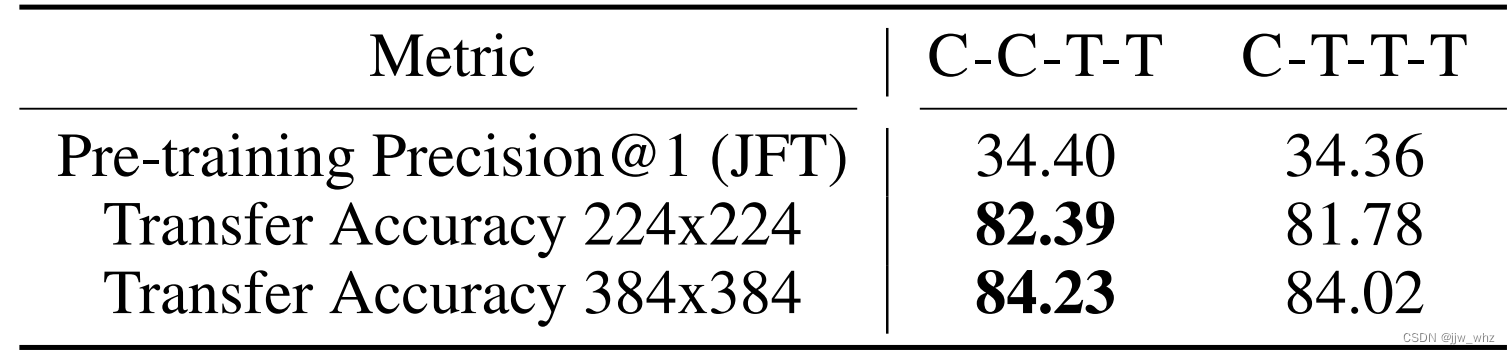

     Last , In order to be in C-C-T-T and C-T-T-T Make a decision in , We arranged another migration test — We are ImageNet-1K Fine tune up two JFT Pre training model 30 round , Compare their migration performance . From the table 2 Look up , It shows C-C-T-T Than C-T-T-T Better migration accuracy , Although the pre training performance is the same .
     Considering the generalization ability , Model performance , Migration capability , And efficiency , We are CoAtNet Adopted C-C-T-T Multistage layout . See the appendix for more details A.1.

3、 Related work

Convolution network building block Convolution network (ConvNets) It is the main neural architecture of many computer vision tasks . Conventional , Conventional convolution image ResNet It is very popular in large-scale convolutional networks . by comparison , Deep convolution is popular on mobile platforms , Because it has lower calculation cost and smaller parameter quantity . Recent work shows that , An improved inversion residual bottleneck (MBConv) It is based on deep convolution , That is, it can achieve high precision , It can also achieve high efficiency . As discussed in part II , because MBConv and Transformer There is a strong connection between the blocks , This paper mainly uses MBConv As a convolution building block .
Self attention and Transformers Under the action of self attention of key elements ,Transformers It is widely used in naturallanguageprocessing , And speech recognition . As an early job , The independent self attention network shows that the independent self attention network can do well in different visual tasks , Despite some practical difficulties . lately , ViT Apply a common Transformer To ImageNet Classification task , On a large scale JFT After pre training on the data set, an impressive result was achieved . However , When the training data set is limited ViT It still lags far behind the best convolutional neural network . Based on this , A lot of recent work has focused on improving vision Transformers Data efficiency and model efficiency . In order to vision Transformers There is a broader review , We recommend that readers refer to a special survey [36, 37].
Relative attention Under the general term of relative attention , There are many variations [30, 38, 39, 34, 40, 31]. generally speaking , We can divide it into two categories ：(a) Input dependent version its additional relative attention score is an input state function $f(x_i,x_j,i-j)$. (b) The input dependent version is $f(i-j)$. CoAtNet The variants of are input dependent versions and T5 One of them is similar to , But with the T5 The difference is , We do not share relative attention parameters across layers nor use the bucket mechanism . One benefit of input independence is in all $(i,j)$ Get... In alignment $f(i-j)$ Than in TPU Lower computational cost for input dependent versions on . besides , In reasoning , This only needs to be calculated once and cached for future use . A recent work has also unified an input dependent parameter , But it limits the receptive field to a local window .
Combine convolution with self attention The idea of combining convolution and self attention is not new to visual recognition tasks . A general approach to enhance the skeleton of convolutional neural networks is ： Replace some convolution layers with explicit self attention or nonlocal modules or standard self attention or flexibly mix attention and convolution linearly . Although self - attention is often used to improve accuracy , But they often have additional computational costs , therefore , Often seen as ConvNets Add on for , Be similar to squeeze-and-excitation modular . by comparison , stay ViT and ResNet-ViT After the successful application of , Another popular research direction is Transformer The backbone network attempts to Transformer Add explicit convolution or some valuable properties of convolution to the backbone network .
     Although our work falls into this category , But our relative attention instantiation is a natural mixture of deep convolution and content-based attention , With a small additional cost . what's more , From the perspective of generalization ability and model performance , We adopt a systematic approach to vertical layout design , And explain how and why different types of layers are used in different network phases . therefore , With those who simply use off the shelf convolution networks such as ResNet-ViT As compared with the trunk layer, when the overall size increases CoAtNet There will also be large-scale convolution stages . per contra , Compared with the model using local attention CoAtNet stay S3 and S4 Use full attention all the time , To ensure the performance of the model , because S3 Takes up most of the calculations and parameters .

4、 experiment

     In this part , We compared... Under comparable settings CoAtNet And the results of previous models . For completeness , All the super parameters are not mentioned here , But in the appendix A.2 Can be viewed in .

4.1、 Experimental setup

Table 3: L Indicates the number of modules ,D Indicates hidden dimension ( Or the number of channels ), For all Conv and MBConv block , We all use a core size of 3 The core of . For all Transformer block , We are in accordance with the [22] Set the size of each attention head to 32. The expansion rate of the inverted bottleneck is 4,SE The expansion of （ shrinkage ） Rate is 0.25.

CoAtNet Model family To compare with existing models of different sizes , We also designed a model family , Table 3 is an overview of the family . in general , from S1 to S4 The number of channels doubles at each stage , At the same time, ensure that the trunk S0 Width ratio of S1 Smaller or equal to . Again , In order to simplify the , As the depth of the network increases , We only in S2 and S3 Number of scaling blocks .
Evaluation protocol Our experiment focuses on image classification , In order to evaluate the performance of the model on different data set sizes , We used three larger and larger datasets , namely ImageNet-1K (128 Ten thousand pictures ), ImageNet-21K (1270 Ten thousand pictures ) and JFT (3 Billion pictures ). According to the previous work , We first use on three data sets 224 The pixels are pre trained respectively 300, 90 and 14 round , then , We are ImageNet-1K The pre training model is tested with the desired resolution 30 Fine adjustment of the wheel , Obtain corresponding evaluation accuracy . One exception is ImageNet-1K At a resolution of 224 You can directly obtain the pre training results . Be careful , And use Transformer Other models of the block are similar , Without fine tuning , With higher resolution directly in ImageNet-1K Evaluating the pre - training model usually leads to performance degradation . therefore , No matter how the input resolution changes , Always use fine tuned .
Data enhancement and regularization In this paper , We only considered two widely used data enhancement methods , Random data enhancement and mixed data enhancement , And three general technologies including ： Random depth , The label is smooth , Weight decline , To regularize the model , Intuitively speaking , Explicit data enhancement and regularization methods depend on the size of the model and the size of the data , Among them, strong regularization is usually applied to larger models and smaller data sets .
     Under normal circumstances , A complex problem under the current paradigm is how to adjust the regularization of pre training and fine tuning with the change of data size . Special , We have an interesting observation , If a certain type of enhancement is completely disabled during pre training , Simply turning it on during fine-tuning is likely to damage performance , Instead of improving performance . We speculate that this may be related to the transfer of data distribution . Final , At some runtime of the proposed model , We are deliberately in two larger ImageNet21-K and JFT A small range of random enhancement and random depth enhancement are used for pre training on the data set . Although such regularization may damage the pre Training Index , But this allows for more regularization and data enhancement during tuning , Thus, the downstream performance is improved .

4.2、 The main result

Table 4: stay ImageNet. 1K Model performance on , Note that training is only in ImageNet-1K On ;21K+1K It means to train in ImageNet-21K, stay ImageNet-1K Fine tune up ; PT-RA Mean in 21K Use random reinforcement during pre training ,E150 Mean in 21K Pre training 150 round , This is better than the standard 90 Long wheel . See the appendix for more results A.3.

Figure 2: Only set to 224x224 stay ImageNet-1K Precision on the surface - Floating point quantity proportional curve .

ImageNet-1K Table 4 shows that only ImageNet-1K Experimental results on datasets . Under the same conditions , What we are talking about CoAtNet The model not only excels ViT Variants , And can rival the best only based on convolution architecture , for example EfficientNet-V2 and NFNets. besides , We are on the table 2 Will also be in 224x224 All results at resolution are visualized . As we can see , With attention module CoAtNet Much better than the previous model .

Figure 3: stay ImageNet-21K Go to pre training and move to ImageNet-1K The precision of the upper trim - Proportional curve of parameter quantity .
ImageNet-21K As we can see from the table 4 As shown in Figure 3 , When in ImageNet-21K When pre training on . CoAtNet The advantage of has become very obvious , It is basically better than all previous models . It is worth noting that , first-class CoAtNet The variant of has reached 88.56% Of top-1 precision . And ViT-H/14 Of 88.55% Compete with , This requires more than CoAtNet Big 2.3 Times ViT-H/14 In comparison ImageNet-21K Big 23 Times if the label data set JFT Pre training is better than in ImageNet-21K Upper 2.2 Times more rounds . This marks a dramatic improvement in data efficiency and computational efficiency .
Table 5: On a large scale JFT Performance comparison on datasets ,TPUv3-core-days Indicates the pre training time ,Top-1 Accuracy It means that ImageNets Fine tuning accuracy on . Be careful : The last three lines are in a larger data set JFT-3B Pre training on , Others are in JFT-300M On .CoAtNet-5/6/7 See the appendix for the size details A.2. stay MBConv The downsampling in the block is done in steps of 2 The depth convolution of .ViT-G/14 The calculation cost of is shown in [26] Figure 1 of this paper .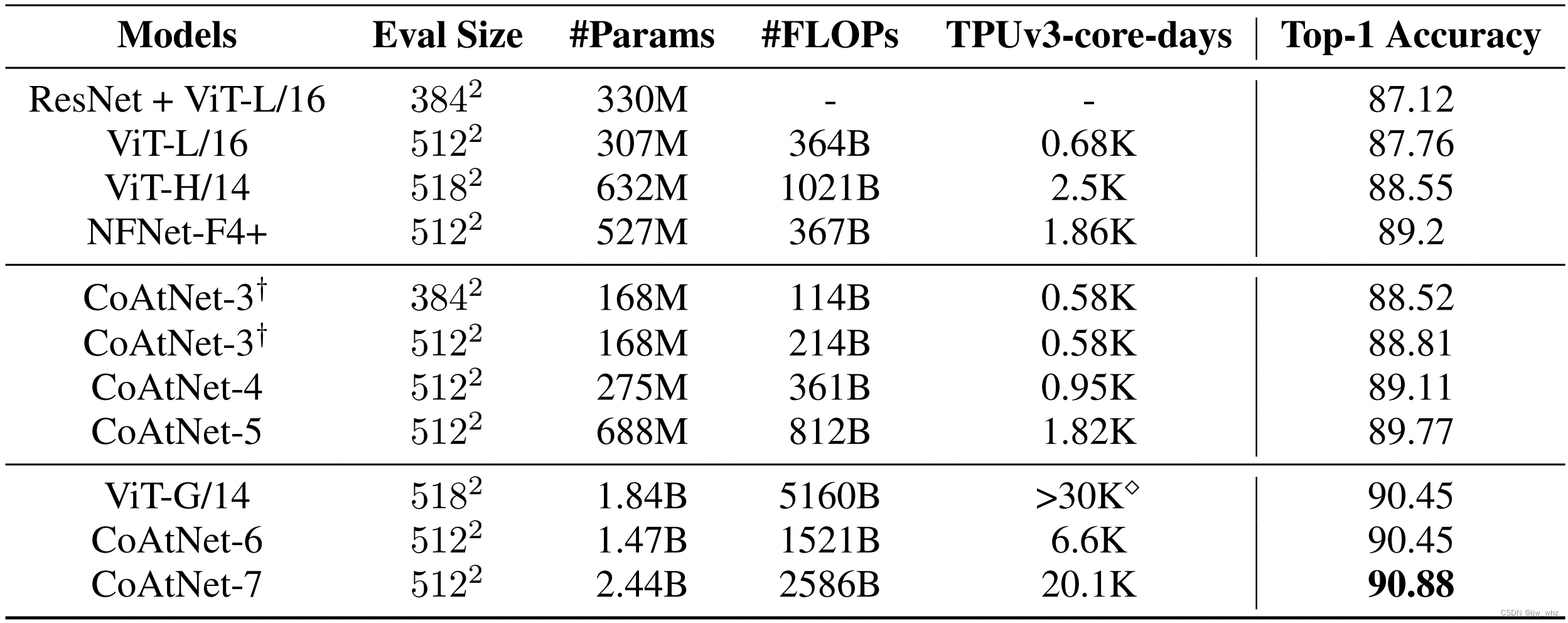

JFT Last , In the table 5 in , In large datasets JFT-300M and JFT-3B Further evaluation on CoAtNet. What is encouraging is , our CoAtNet-4 By setting NFNet-F4+ stay JFT-300M Can match the previous best performance and the efficiency is TPU It is twice as long as the training time and parameters . When we enlarge the model to the same training resources, such as NFNet-F4+, CoAtNet-5 Reached 89.77% Of top-1 precision , Outperforms previous results in comparable settings .
     and , As we further put our training resources into ViT-G/14 The level of use , Use a larger JFT-3B Data sets , More than four times the amount of computation , CoAtNet-6 Is able to ViT-G/14 Of 90.45% A match , have 1.5 Times less computation ,CoAtNet-7 Reached 89.77% top-1 Accuracy of 90.88%, It has reached the new best performance at present .

4.3、 Melting research

     In this part , We are going to CoAtNet Do ablation experiments .

                                                                    Table 6: Ablation experiments on relative attention

     First , We study the importance of relative attention by integrating convolution and attention into a computing unit . Special , We compare the two models , One with relative attention , The other didn't , Both are alone ImageNet-1K and ImageNet-21K Make migration settings on . As we can see from table 6 , When only with ImageNet-1K when , Relative attention clearly outperforms standard attention , Have better generalization ability . besides , stay ImageNet-21K Migration settings , The relative attention variant achieves a better transfer accuracy , Although their pre training performance is close to . This shows that the main advantage of relative attention in visual processing is not only higher performance , And it has better generalization ability .
                                                                    Table 7: Ablation Experiment on architecture layout

     second , Because with MBConv The block S2 And have relative Transformer The block S3 Account for the CoAtNet The main calculation of . One problem is how to segment in S2 (MBConv) and and S3 (Transformer) To achieve a good computing performance . In practice , It is determined by the number of blocks in each phase , We call it “ Layout ” Design . For this question , We compared some different layouts . The experimental results are shown in Table 7 .

• If we keep at S2 and S3 The total number of blocks in is fixed , We observed that V0 yes V1 and V2 The best point between . On the whole ,S3 There are more of them Transformer Blocks usually lead to better performance , until S2 in MBConv The number of blocks is too small to be generalized well .
• Further evaluate whether there is an optimal point in the migration settings , It is generally considered that higher performance is more important , We further compare the results from ImageNet-21K Migrate to ImageNet-1K Under settings V0 and V1. What's interesting is that , Even though V1 and V0 stay ImageNet-21K Same performance during pre training , however V1 The migration accuracy of is significantly lower than V0. This shows the importance of convolution in achieving better migration and generalization capabilities .

                                              Table 7: Ablation experiments on attentional head size and normalized type

     Last , We studied the details of the two selected models , That is to say MBConv Dimension and normalized type of each attention head in the block . From the table 8 We can see that as the number of attention heads increases from 32 Add to 64 Slightly detrimental to performance , Although it actually greatly improves TPU The speed of . actually , This will be a quality - Speed tradeoff . On the other hand , Batch normalization and Layer normalization has almost the same performance , and TPU Upper BatchNorm Speed up 10-20%, It depends on the batch size of each core .

5、 Conclusion

     In this paper , We systematically study convolution and Transformers Properties of , This gives rise to a rule , Combine them into one called CoAtNet A new family of models . Extended experiments show that CoAtNet Have the image ConvNets This good generalization ability is similar to that of Transformers Such supervised model performance , At different data sizes and computing costs, it achieves the best performance at present .
     Be careful , At present, this paper mainly focuses on ImageNet classification . However , We believe that our method is applicable to a wider range of applications , Such as target detection and semantic segmentation . We will leave them to future work .