The beautiful scenery is natural, and the wonderful pen is obtained by chance -- how is the "wonderful pen" refined?

Project background

The opening ceremony of the Winter Olympics just passed , It can be said to be a beautiful visual feast . among , The combination of technology and art has created various dreamy visual effects , Let's see AI There is much to be done in the field of art . And the project shared today is also AI+ A small direction of art , Inspired by my little daughter .

One day , My little daughter said ：“ Dad , I want to be a cartoonist when I grow up , Today I'm going to draw Dora A dream ！”. It's very comforting , They don't have to be like me and my parents when they were young , To learn well is to travel all over the world “ Not afraid of ”, They study just because “ like ”. But , It is not so easy to like . After half a day's training “ Waving ink in the air ”,“ Little cartoonist ” I always feel that my paintings are Dora A Dreams are not as good-looking as books , Gradually a little discouraged . Seeing children's dreams have not taken off , Wings are about to break , All blame the steep learning curve . I suddenly remembered a man named GauGAN Model of , Can edit pictures according to image semantics . that , Why not use this model to make a graffiti game , Let the children be like little Ma Liang “ A good pen makes a good picture ” Well ？

Technology is introduced

The graffiti application model introduced in this paper is from the article 《Semantic Image Synthesis with Spatially-Adaptive Normalization》. This model has a nice name GauGAN [1] ,Gau It's van Gogh's Gau, In style migration network Pix2PixHD Has been improved on the generator of , Use SPADE（Spatially-Adaptive Normalization） Module replaces the original BN layer , In order to solve the problem that the picture feature map passes through BN Layer when the information is “ Wash off ” The problem of .Pix2PixHD It's actually a CGAN（Conditional GAN） Conditional generation countermeasure network , It can be controlled by entering the tag , That is, the semantic segmentation mask controls the content of each part of the generated image . Here is a detailed introduction GauGAN Implementation details of each component .

1. Multiscale discriminator

（Multi-scale discriminators）

So-called “ Multiscale ” Judging device , Is to make multiple structures the same 、 A group of discriminators with different sizes of input feature map are fused together for use . When judging pictures , First, the pictures are scaled to different sizes and sent to these discriminators , Then the outputs of these discriminators are weighted and added to obtain the final discriminating output , This can enhance the discriminating ability of the discriminator , Make the output of the generator more realistic .

# Multi-scale discriminators  Discriminator code class MultiscaleDiscriminator(nn.Layer):    def __init__(self, opt):        super(MultiscaleDiscriminator, self).__init__()        for i in range(opt.num_D):            sequence = []            feat_size = opt.crop_size            for j in range(i):                sequence += [nn.AvgPool2D(3, 2, 1)]                feat_size = np.floor((feat_size + 1 * 2 - (3 - 2)) / 2).astype('int64') #  Calculate the scaling ratio of each discriminator input             opt_downsampled = copy.deepcopy(opt)            opt_downsampled.crop_size = feat_size            sequence += [NLayersDiscriminator(opt_downsampled)]            sequence = nn.Sequential(*sequence)            self.add_sublayer('nld_'+str(i), sequence)    def forward(self, input):        output = []        for layer in self._sub_layers.values():            output.append(layer(input))        return output

The integrated discriminators input images with different scaling scales to calculate the discrimination results , Zoom through feat_size = np.floor((feat_size + 1 * 2 - (3 - 2)) / 2).astype('int64') To calculate the .

2. Gradually refined generator

（Coarse-to-fine generator）

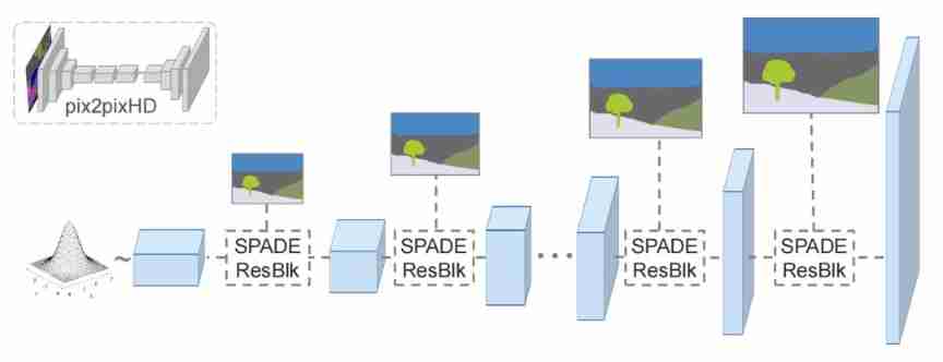
The idea of the generator is similar to that of the discriminator , First train a low resolution generator , And then train with a high-resolution generator . When training the high score generator, use the characteristic graph of the low score generator as an auxiliary .Pix2PixHD The generator of the model inputs semantic tags , Output photo style pictures , So it has a complete “Encoder-Decoder（ codecs ） structure ”, and GauGAN The generator of the model only needs to input a random noise with normal distribution , The encoder part is not required . Their structural comparison is shown in the following figure ：

# Coarse-to-fine generator  Generator code class SPADEGenerator(nn.Layer):    def __init__(self, opt):        super(SPADEGenerator, self).__init__()        self.opt = opt        nf = opt.ngf        self.sw, self.sh = self.compute_latent_vector_size(opt)        if self.opt.use_vae:            self.fc = nn.Linear(opt.z_dim, 16 * opt.nef * self.sw * self.sh)            self.head_0 = SPADEResnetBlock(16 * opt.nef, 16 * nf, opt)        else:            self.fc = nn.Conv2D(self.opt.semantic_nc, 16 * nf, 3, 1, 1)            self.head_0 = SPADEResnetBlock(16 * nf, 16 * nf, opt)        self.G_middle_0 = SPADEResnetBlock(16 * nf, 16 * nf, opt)        self.G_middle_1 = SPADEResnetBlock(16 * nf, 16 * nf, opt)        self.up_0 = SPADEResnetBlock(16 * nf, 8 * nf, opt)        self.up_1 = SPADEResnetBlock(8 * nf, 4 * nf, opt)        self.up_2 = SPADEResnetBlock(4 * nf, 2 * nf, opt)        self.up_3 = SPADEResnetBlock(2 * nf, 1 * nf, opt)        final_nc = nf        if opt.num_upsampling_layers == 'most':            self.up_4 = SPADEResnetBlock(1 * nf, nf // 2, opt)            final_nc = nf // 2        self.conv_img = nn.Conv2D(final_nc, 3, 3, 1, 1)        self.up = nn.Upsample(scale_factor=2)    def forward(self, input, z=None):        seg = input        if self.opt.use_vae:            x = self.fc(z)            x = paddle.reshape(x, [-1, 16 * self.opt.nef, self.sh, self.sw])        else:            x = F.interpolate(seg, (self.sh, self.sw))            x = self.fc(x)        x = self.head_0(x, seg)        x = self.up(x)        x = self.G_middle_0(x, seg)        if self.opt.num_upsampling_layers == 'more' or \           self.opt.num_upsampling_layers == 'most':            x = self.up(x)        x = self.G_middle_1(x, seg)        x = self.up(x)        x = self.up_0(x, seg)        x = self.up(x)        x = self.up_1(x, seg)        x = self.up(x)        x = self.up_2(x, seg)        x = self.up(x)        x = self.up_3(x, seg)        if self.opt.num_upsampling_layers == 'most':            x = self.up(x)            x = self.up_4(x, seg)        x = self.conv_img(F.gelu(x))        x = F.tanh(x)        return x

The generator without encoder part is composed of head（0）,G_middle（0,1） and up(0,1,2,3） Three parts .head It mainly deals with generator input noise . If you use VAE（ Variational self encoder ） Generate multiple models , The input is VAE Extracted from feature pictures latent code（ Latent variable ）, To control the style of the output picture . Two layers of G_middle Handle feature mapping .4 layer up（ or 5 layer , Depending on the output size ） Sample the feature map layer by layer , Until the output dimension is reached .

To further improve the quality of the generated image , The model also adds... To the generator Instance Map（ Instance split label ） As a control variable ：

With Instance Map Edge information provided , The edges of different objects of the same type in the image generated by the model are more clear and reasonable , As shown by the edge of adjacent cars in the above figure .

3. Spatial adaptive normalization SPADE

（Spatially-Adaptive Normalization）

In order to solve Pix2PixHD When generating photo style images through semantic tags , The characteristic information is represented by a normalization layer “ Wash off ” The problem of ,GauGAN Put forward Spatially-Adaptive （De）Normalization, namely “ Spatial adaptation （ back ） normalization ”, abbreviation SPADE.

SPADE The module will input the semantic tags separately embedding To two convolution layers , Then the two convolution layers which retain the spatial information of semantic labels are used to replace the scaling coefficients and offsets in the original normalization layer . Use SPADE The comparison before and after the module is shown in the following figure ：

The contrast shows , With SPADE Module blessings , The style migration network is no longer afraid to convert large semantic tags . therefore , This model of generating pictures by semantic mask is also called “ Semantic image synthesis network ”.

# SPADE Space adaptive normalization module code class SPADE(nn.Layer):    def __init__(self, config_text, norm_nc, label_nc):        super(SPADE, self).__init__()        parsed = re.search(r'spade(\D+)(\d)x\d', config_text)        param_free_norm_type = str(parsed.group(1))        ks = int(parsed.group(2))        self.param_free_norm = build_norm_layer(param_free_norm_type)(norm_nc) #  This process must turn off the adaptive parameters of the normalization layer         # The dimension of the intermediate embedding space. Yes, hardcoded.        nhidden = 128        pw = ks // 2        self.mlp_shared = nn.Sequential(*[            nn.Conv2D(label_nc, nhidden, ks, 1, pw),            nn.GELU(),        ])        self.mlp_gamma = nn.Conv2D(nhidden, norm_nc, ks, 1, pw)        self.mlp_beta = nn.Conv2D(nhidden, norm_nc, ks, 1, pw)    def forward(self, x, segmap):        # Part 1. generate parameter-free normalized activations        normalized = self.param_free_norm(x)        # Part 2. produce scaling and bias conditioned on semantic map        segmap = F.interpolate(segmap, x.shape[2:])        actv = self.mlp_shared(segmap)        gamma = self.mlp_gamma(actv)        beta = self.mlp_beta(actv)        # apply scale and bias        out = normalized * (1 + gamma) + beta        return out

SPADE The module first turns off the adaptive scaling coefficient and offset of the normalization layer , Then the scaled feature map （ To adapt to the output of different sizes of the previous layer ）embedding To mlp_gamma In the convolution layer , Then map to gamma Convolution layer （ The zoom ） and beta Convolution layer （ bias ）, That's it “ use 2d Convolution layer replacement replaces scalar scaling coefficients and offsets ” The operation of , To save “ adopt BN Spatial information of layers ” Purpose .

4.GauGAN Of Loss Calculation

（hinge Loss、Feat Loss、Perceptual Loss）

GauGAN The multi-scale discriminator not only integrates multiple scaled size discriminators , And in calculating and judging Loss when , Not only the output of the last layer is calculated , The characteristic graph output from the middle layer of the discriminator also participates in Loss Calculation , The formula is as follows ：

Pix2PixHD Also used. ImageNet Pre trained on dataset VGG19 The model is calculated as an additional feature extractor Perceptual Loss, Used to compare true and false pictures . With the use of discriminator middle layer output characteristic graph calculation Loss Time is different , Use VGG19 Calculation of middle layer characteristic diagram Loss It should be weighted layer by layer , Make the model more sensitive to high-level semantic features .

GauGAN Of Loss from “ Against the loss ”、“ Discriminator auxiliary loss ” and “ Generator auxiliary loss ” Three parts .

① To counter the loss, use Hinge Loss

#  Discriminator against loss df_ganloss = 0.for i in range(len(pred)):    pred_i = pred[i][-1][:batch_size]    new_loss = -paddle.minimum(-pred_i - 1, paddle.zeros_like(pred_i)).mean() # hingle loss    df_ganloss += new_lossdf_ganloss /= len(pred)dr_ganloss = 0.for i in range(len(pred)):    pred_i = pred[i][-1][batch_size:]    new_loss = -paddle.minimum(pred_i - 1, paddle.zeros_like(pred_i)).mean() # hingle loss    dr_ganloss += new_lossdr_ganloss /= len(pred)#  Generator against loss g_ganloss = 0.for i in range(len(pred)):    pred_i = pred[i][-1][:batch_size]    new_loss = -pred_i.mean() # hinge loss    g_ganloss += new_lossg_ganloss /= len(pred)

df_ganloss and dr_ganloss It is to distinguish the false picture and the true picture Loss,g_ganloss Is the generator loss . Use hinge loss When calculating the discriminator loss , Only the loss of some samples is used to update the gradient each time , Stable generator updates . therefore , The later improved model even removed the spectral normalization layer used to update the stability discriminator .

② The auxiliary loss of the discriminator is calculated by using the characteristic graph output from the middle layer of the discriminator L1 Loss Add and make

g_featloss = 0.for i in range(len(pred)):    for j in range(len(pred[i]) - 1): #  Remove the middle layer of the last layer featuremap        unweighted_loss = (pred[i][j][:batch_size] - pred[i][j][batch_size:]).abs().mean() # L1 loss        g_featloss += unweighted_loss * opt.lambda_feat / len(pred)

③ Generator auxiliary loss of use VGG19 The characteristic graph output from the middle layer of the pre training model is weighted layer by layer L1 Loss Add and make

g_vggloss = paddle.to_tensor(0.)if not opt.no_vgg_loss:    rates = [1.0 / 32, 1.0 / 16, 1.0 / 8, 1.0 / 4, 1.0]    _, fake_features = vgg19(resize(fake_img, opt, 224))    _, real_features = vgg19(resize(image, opt, 224))    for i in range(len(fake_features)):        g_vggloss += rates[i] * l1loss(fake_features[i], real_features[i])    g_vggloss *= opt.lambda_vgg

④GauGAN The total loss function

Discriminator total loss function ：

d_loss = df_ganloss + dr_ganloss

Generator total loss function ：

if opt.use_vae:    g_loss = g_ganloss + g_featloss + g_vggloss + g_vaeloss    opt_e.clear_grad()    g_loss.backward(retain_graph=True)    opt_e.step()else:    g_loss = g_ganloss + g_featloss + g_vgglossopt_g.clear_grad()g_loss.backward()opt_g.step()

If you use VAE Control the style of the generated picture , Plus VAE The generated variational distribution and Gaussian prior distribution KL Divergence calculation g_vaeloss, To narrow the style similarity between the input image and the generated image .

Engineering practice and more exploration

1. Some problems encountered in project implementation

① Data processing

CycleGAN I once roast when I raised it Pix2Pix This pixel style migration model relies heavily on paired datasets . however , fortunately “ Image segmentation ” As CV Learn more about the three swordsmen （ Image classification 、 object detection 、 Image segmentation ） One of , A large number of training data sets and pre training models can be used “ Style transfer / Semantic image synthesis ” Tasks .

Training “ A good pen makes a good picture ” The data you need can be annotated using the split model . First , Use Flying propeller Target detection kit PaddleDetection stay ade20k Training a segmentation model on a dataset , This segmentation model can then be used to annotate landscape images obtained from other data sets or resources . Of course , If there is a pre training model , It can also be used directly , As long as the classification category is processed accordingly . except ade20k Segmentation model trained on , I think coco The training on the data set should also be able to use .

The accuracy of the segmentation model used to label data is not very high , But the marked data seems to have a good effect . Maybe when generating a model to fit the probability distribution , Those pixels with low frequency of wrong annotation are not displayed , If you use the way of clipping channels to compress the model , Those low probability misexpressions are even cut out .

② Deploy

“ A good pen makes a good picture ” The background of is to use Flying propeller Pre training model application tool PaddleHub The deployment of , The front-end display page uses H5 Written Web page , This is what we have to deal with JavaScript The problem of script cross domain access . The current project is still through a relay PHP The server script has been transferred http request , But this will lead to a relatively large burden of data transmission . If you can set up cross domain resource sharing on the server （CORS） White list to address cross domain access , It is more efficient . Methods are still being explored , Welcome to the discussion .

2. Model improvement and ongoing follow-up processing

① Add attention

Now? , Attention is very popular , But semantic image synthesis is far from the top Transfomer It's a little far away , Then use it first 21 year “ Up to date ” Of SimAM（Simple, Parameter-Free Attention Module Simple nonparametric attention module ） Try it . This attention mechanism draws on neuroscience theory , Use the energy function to evaluate the importance of neurons . The code is as follows ：

def simam(x, e_lambda=1e-4):    b, c, h, w = x.shape    n = w * h - 1    x_minus_mu_square = (x - x.mean(axis=[2, 3], keepdim=True)) ** 2    y = x_minus_mu_square / (4 * (x_minus_mu_square.sum(axis=[2, 3], keepdim=True) / n + e_lambda)) + 0.5    return x * nn.functional.sigmoid(y)

Sure enough Simple,6 Line code （ Code above ）. This SimAM The module is added after the activation of each residual of the generator and discriminator , For detailed settings, please refer to the AI Studio Open source project . The picture below is GauGAN Use SimAM Contrast before and after attention （ The left column is for use SimAM after , The second column on the left is the original GauGAN, The three columns on the left are real pictures , The three columns on the right are deeplabv2 The segmentation result of the pre training model ）.

② upgrade SPADE modular

SPADE The module is easy to use , But the cost of calculation is huge , therefore , Someone produced a simplified version of “ The adaptive （ back ） Normalization module ”

The starting idea is ： What really makes the model more effective is SPADE Category information retained in the module , Space, not information . therefore , An improved version of CLADE（Class-Adaptive（De）Normalization） The module only maps the category information to the scaling coefficient and offset of the inverse normalization module , It greatly saves the amount of parameters and calculation . But then I found out , Preserving spatial information can improve the effect of the model , Then we use semantic tags to calculate manually ICPE（intra-class positional encoding In class location embedding code ） Multiplied by the scaling factor and the offset . The final version of CLADE-ICPE Between build quality and SPADE Quite often , It greatly reduces the amount of parameters and calculation .

③ Compression model

‍‍‍‍‍‍‍‍‍‍‍ Except yes SPADE The module is improved , Recently, I published two more compressed articles GAN Model article , Is also experimenting , A brief introduction .‍‍‍‍‍‍‍‍‍‍‍

GAN CAT（Compression And Teaching Compression and distillation ）

GAN CAT The greatest feature of the method is ： Teacher builder TeacherG Except for distillation , Also used as a model search space , No extra training is required Supernet Model . The search space of the model structure is through InsResBlocks Module implementation . The clipping process selects both the model structure and the channel .

CAT Method to crop the threshold used （ Scaling factor of normalization layer ） Automatically calculate according to the compression target , There is no need to iterate the clipping process . Distillation uses KA（Kernel Alignment） Measure the similarity between convolution structures with different channel numbers .

OMGD（Online Multi-Granularity Distillation Multi particle online distillation ）

OMGD Our thinking is very clear , Is to use a deeper model and a wider model to distill , A picture to cover it ：

OMGD Train two deeper 、 Wider teacher builder , While distilling , It can make the process more stable , This is online . When a teacher model with the same depth and wider width is used for distillation ,loss Function not only compares the output , Moreover, the characteristic diagram of the middle layer is also used Structural Similarity (SSIM) Loss compare , So it is called multi granularity .

Conclusion

Last , Let's see “ A wonderful pen ” What is it? “ Raw painting ” . ：

In the near future , More coquettish GauGAN2‍‍‍‍‍‍‍ Released , Eight kinds of martial arts SOTA Nuwa of also released , even to the extent that StyleGAN I dare to undertake any task , It all went wrong , Visually check that a large wave of interesting models are coming in front , Let us in the metauniverse happy Big land GAN Let's have a fight ！

In order to facilitate everyone to experience all kinds of GAN Model , Here are some sent to AI Studio The open source project on ：

①GAN Of “ Five parts of style transfer ”

• 《 Understand the classic of generating confrontation network GAN》 https://aistudio.baidu.com/aistudio/projectdetail/551962

• 《 Article, understand GAN The style of Conditional GAN》 https://aistudio.baidu.com/aistudio/projectdetail/644398

• 《 Article, understand GAN The style of Pix2Pix》 https://aistudio.baidu.com/aistudio/projectdetail/1119048

• 《 Article, understand GAN The style of CycleGAN》 https://aistudio.baidu.com/aistudio/projectdetail/1153303

• 《 Article, understand GAN The style of SPADE Paper recurrence 》

  https://aistudio.baidu.com/aistudio/projectdetail/1964617

• 《 A good pen makes a good picture 》

  https://aistudio.baidu.com/aistudio/projectdetail/2274565

②GAN“ Prequel ”

• 《 One article to understand convolution network （ from LeNet To GoogLeNet）》 https://aistudio.baidu.com/aistudio/projectdetail/601071

• 《 Hands-on deep learning 》Paddle Version source code （ classic CV Network collection ） https://aistudio.baidu.com/aistudio/projectdetail/1639856

reference

[1] Park T, Liu M Y, Wang T C, et al. Semantic Image Synthesis With Spatially-Adaptive Normalization[C]// 2019 IEEE/CVF Conference on Computer Vision and Pattern Recognition (CVPR). IEEE, 2019.

Official account , Get more technical content ~

This article is shared in Blog “ Flying propeller PaddlePaddle”（CSDN）.
If there is any infringement , Please contact the [email protected] Delete .
Participation of this paper “OSC Source creation plan ”, You are welcome to join us , share .