当前位置:网站首页>Least squares system identification class II: recursive least squares
Least squares system identification class II: recursive least squares
2022-06-26 16:16:00 【RuiH. AI】
Least squares system identification class medium-length : Recursive least squares
Preface
This paper records the principle of recursive least squares in the course of system identification .
Least squares estimate
The following system identification model :
{ y ( 1 ) = φ T ( 1 ) θ + v ( 1 ) y ( 2 ) = φ T ( 2 ) θ + v ( 2 ) . . . y ( t ) = φ T ( t ) θ + v ( t ) set up : Y t = [ y ( 1 ) y ( 2 ) . . . y ( t ) ] T H t = [ φ ( 1 ) φ ( 2 ) . . . φ ( t ) ] T V t = [ v ( 1 ) v ( 2 ) . . . v ( n ) ] T Yes : Y t = H t θ + V t \left \{ \begin{aligned} y(1)&=\varphi^T(1)\theta+v(1) \\ y(2)&=\varphi^T(2)\theta+v(2) \\ &... \\ y(t)&=\varphi^T(t)\theta+v(t) \end{aligned} \right . \\ \quad \\ \begin{aligned} set up : Y_t&=[y(1)\quad y(2)\quad ... \quad y(t)]^T \\ H_t&=[\varphi(1) \quad \varphi(2) \quad ... \quad \varphi(t)]^T \\ V_t&=[v(1) \quad v(2) \quad ... \quad v(n)]^T \end{aligned} \\ \quad \\ Yes : Y_t=H_t\theta +V_t ⎩⎪⎪⎪⎪⎨⎪⎪⎪⎪⎧y(1)y(2)y(t)=φT(1)θ+v(1)=φT(2)θ+v(2)...=φT(t)θ+v(t) set up :YtHtVt=[y(1)y(2)...y(t)]T=[φ(1)φ(2)...φ(t)]T=[v(1)v(2)...v(n)]T Yes :Yt=Htθ+Vt
The least square estimation of parameters can be expressed as :
θ ^ L S = ( H t T H t ) − 1 H t T Y t \hat\theta_{LS}=(H_t^TH_t)^{-1}H_t^TY_t θ^LS=(HtTHt)−1HtTYt
The above method updates the input and output data at each new time , Must be re estimated , The computational load is heavy .
Recursive least squares estimation
principle
Recursive least square estimation uses incremental method , The following is derived :
P − 1 ( t ) = H t T H t = ∑ i = 1 t φ ( i ) φ T ( i ) = ∑ i = 1 t − 1 φ ( i ) φ T ( i ) + φ ( t ) φ T ( t ) = P − 1 ( t − 1 ) + φ ( t ) φ T ( t ) θ ^ ( t ) = ( H t T H t ) − 1 H t T Y t = P ( t ) H t T Y t = P ( t ) [ H t − 1 T φ ( t ) ] [ Y t − 1 T y ( t ) ] T = P ( t ) H t − 1 T Y t − 1 T + P ( t ) φ ( t ) y ( t ) = P ( t ) P − 1 ( t − 1 ) P ( t − 1 ) H t − 1 T Y t − 1 T + P ( t ) φ ( t ) y ( t ) = P ( t ) P − 1 ( t − 1 ) θ ^ ( t − 1 ) + P ( t ) φ ( t ) y ( t ) = P ( t ) [ P − 1 ( t ) − φ ( t ) φ T ( t ) ] θ ^ ( t − 1 ) + P ( t ) φ ( t ) y ( t ) = θ ^ ( t − 1 ) − P ( t ) φ ( t ) φ T ( t ) θ ^ ( t − 1 ) + P ( t ) φ ( t ) y ( t ) = θ ^ ( t − 1 ) + P ( t ) φ ( t ) [ y ( t ) − φ T ( t ) θ ^ ( t − 1 ) ] lead The reason is : Moment front A , B , C , if ( I + C A − 1 B ) And A all can The inverse , be : ( A + B C ) − 1 = A − 1 − A − 1 B ( I + C A − 1 B ) − 1 C A − 1 P − 1 ( t ) = P − 1 ( t − 1 ) + φ ( t ) φ T ( t ) hold after Noodles Of type Son take The inverse , root According to the lead The reason is Yes : P ( t ) = P ( t − 1 ) − P ( t − 1 ) φ ( t ) φ T ( t ) P ( t − 1 ) 1 + φ T ( t ) P ( t − 1 ) φ ( t ) P ( t ) φ ( t ) = P ( t − 1 ) φ ( t ) 1 + φ T ( t ) P ( t − 1 ) φ ( t ) L ( t ) = P ( t ) φ ( t ) P^{-1}(t)=H_t^TH_t=\sum_{i=1}^t \varphi(i)\varphi^T(i)=\sum_{i=1}^{t-1} \varphi(i)\varphi^T(i) + \varphi(t)\varphi^T(t) = P^{-1}(t-1)+ \varphi(t)\varphi^T(t) \\ \quad \\ \begin{aligned} \hat\theta(t)&=(H_t^TH_t)^{-1}H_t^TY_t \\ &=P(t)H_t^TY_t \\ &=P(t)\begin{bmatrix} H_{t-1}^T & \varphi(t) \end{bmatrix} \begin{bmatrix} Y_{t-1}^T & y(t) \end{bmatrix}^T \\ &=P(t)H_{t-1}^TY_{t-1}^T + P(t)\varphi(t)y(t) \\ &=P(t)P^{-1}(t-1)P(t-1)H_{t-1}^TY_{t-1}^T + P(t)\varphi(t)y(t) \\ &=P(t)P^{-1}(t-1)\hat \theta(t-1)+P(t)\varphi(t)y(t) \\ &=P(t)[P^{-1}(t)- \varphi(t)\varphi^T(t) ]\hat\theta(t-1)+P(t)\varphi(t)y(t) \\ &=\hat\theta(t-1)-P(t)\varphi(t)\varphi^T(t)\hat\theta(t-1)+P(t)\varphi(t)y(t) \\ &=\hat\theta(t-1)+P(t)\varphi(t)[y(t)-\varphi^T(t)\hat\theta(t-1)] \end{aligned} \\ \quad \\ lemma : matrix A,B,C, if (I+CA^{-1}B) And A It's reversible , be :\\ (A+BC)^{-1}=A^{-1}-A^{-1}B(I+CA^{-1}B)^{-1}CA^{-1} \\ \quad \\ P^{-1}(t)= P^{-1}(t-1)+ \varphi(t)\varphi^T(t) \\ \quad \\ Take the inverse of the following formula , According to lemma, there are :\\ P(t)=P(t-1)-\frac{P(t-1)\varphi(t)\varphi^T(t)P(t-1)}{1+\varphi^T(t)P(t-1)\varphi(t)} \\ \quad \\ P(t)\varphi(t)= \frac{P(t-1)\varphi(t)}{1+\varphi^T(t)P(t-1)\varphi(t)} \\ \quad \\ L(t)=P(t)\varphi(t) P−1(t)=HtTHt=i=1∑tφ(i)φT(i)=i=1∑t−1φ(i)φT(i)+φ(t)φT(t)=P−1(t−1)+φ(t)φT(t)θ^(t)=(HtTHt)−1HtTYt=P(t)HtTYt=P(t)[Ht−1Tφ(t)][Yt−1Ty(t)]T=P(t)Ht−1TYt−1T+P(t)φ(t)y(t)=P(t)P−1(t−1)P(t−1)Ht−1TYt−1T+P(t)φ(t)y(t)=P(t)P−1(t−1)θ^(t−1)+P(t)φ(t)y(t)=P(t)[P−1(t)−φ(t)φT(t)]θ^(t−1)+P(t)φ(t)y(t)=θ^(t−1)−P(t)φ(t)φT(t)θ^(t−1)+P(t)φ(t)y(t)=θ^(t−1)+P(t)φ(t)[y(t)−φT(t)θ^(t−1)] lead The reason is : Moment front A,B,C, if (I+CA−1B) And A all can The inverse , be :(A+BC)−1=A−1−A−1B(I+CA−1B)−1CA−1P−1(t)=P−1(t−1)+φ(t)φT(t) hold after Noodles Of type Son take The inverse , root According to the lead The reason is Yes :P(t)=P(t−1)−1+φT(t)P(t−1)φ(t)P(t−1)φ(t)φT(t)P(t−1)P(t)φ(t)=1+φT(t)P(t−1)φ(t)P(t−1)φ(t)L(t)=P(t)φ(t)
therefore , The recursive least squares of the system parameters can be expressed as :
θ ^ ( t ) = θ ^ ( t − 1 ) + L ( t ) [ y ( t ) − φ T ( t ) θ ^ ( t − 1 ) ] ] L ( t ) = P ( t − 1 ) φ ( t ) 1 + φ T ( t ) P ( t − 1 ) φ ( t ) P ( t ) = [ I − L ( t ) φ T ( t ) ] P ( t − 1 ) , P ( 0 ) = p 0 I , p 0 = inf φ ( t ) = [ . . . ] \hat\theta(t)=\hat\theta(t-1)+L(t)[y(t)-\varphi^T(t)\hat\theta(t-1)]] \\ \quad \\ L(t)=\frac{P(t-1)\varphi(t)}{1+\varphi^T(t)P(t-1)\varphi(t)} \\ \quad \\ P(t)=[I-L(t)\varphi^T(t)]P(t-1), P(0)=p_0I, p_0=\inf \\ \quad \\ \varphi(t)=[...] θ^(t)=θ^(t−1)+L(t)[y(t)−φT(t)θ^(t−1)]]L(t)=1+φT(t)P(t−1)φ(t)P(t−1)φ(t)P(t)=[I−L(t)φT(t)]P(t−1),P(0)=p0I,p0=infφ(t)=[...]
New interest , residual
New interest e ( t ) = y ( t ) − φ T ( t ) θ ^ ( t − 1 ) e(t)=y(t)-\varphi^T(t)\hat\theta(t-1) e(t)=y(t)−φT(t)θ^(t−1)
residual ε ( t ) = y ( t ) − φ T ( t ) θ ^ ( t ) \varepsilon(t)=y(t)-\varphi^T(t)\hat\theta(t) ε(t)=y(t)−φT(t)θ^(t)
Data saturation
The phenomenon
When the input-output time series is long enough , The new input and output do not contribute to the result of recursive least squares estimation , It is called data saturation .
reason
P ( t ) = [ P − 1 ( t − 1 ) + φ ( t ) φ T ( t ) ] − 1 = > P ( t ) ≤ P ( t − 1 ) ( α I + 1 / p 0 ) t ≤ P − 1 ( t ) = P − 1 ( 0 ) + ∑ i = 1 t φ ( i ) φ T ( i ) ≤ ( β I + 1 / p 0 ) t lim t − > inf P − 1 ( t ) = 0 P(t)=[P^{-1}(t-1)+\varphi(t)\varphi^T(t)]^{-1} => P(t)\le P(t-1) \\ (\alpha I+1/p_0)t\le P^{-1}(t) = P^{-1}(0)+ \sum_{i=1}^t\varphi(i)\varphi^T(i) \le (\beta I+1/p_0)t \\ \lim_{t->\inf}P^{-1}(t) = 0 P(t)=[P−1(t−1)+φ(t)φT(t)]−1=>P(t)≤P(t−1)(αI+1/p0)t≤P−1(t)=P−1(0)+i=1∑tφ(i)φT(i)≤(βI+1/p0)tt−>inflimP−1(t)=0
resolvent : Recursive least squares with forgetting factor
θ ^ ( t ) = θ ^ ( t − 1 ) + L ( t ) [ y ( t ) − φ T ( t ) θ ^ ( t − 1 ) ] ] L ( t ) = P ( t − 1 ) φ ( t ) λ + φ T ( t ) P ( t − 1 ) φ ( t ) P ( t ) = 1 λ [ I − L ( t ) φ T ( t ) ] P ( t − 1 ) , P ( 0 ) = p 0 I , p 0 = inf φ ( t ) = [ . . . ] \hat\theta(t)=\hat\theta(t-1)+L(t)[y(t)-\varphi^T(t)\hat\theta(t-1)]] \\ \quad \\ L(t)=\frac{P(t-1)\varphi(t)}{\lambda+\varphi^T(t)P(t-1)\varphi(t)} \\ \quad \\ P(t)=\frac{1}{\lambda}[I-L(t)\varphi^T(t)]P(t-1), P(0)=p_0I, p_0=\inf \\ \quad \\ \varphi(t)=[...] θ^(t)=θ^(t−1)+L(t)[y(t)−φT(t)θ^(t−1)]]L(t)=λ+φT(t)P(t−1)φ(t)P(t−1)φ(t)P(t)=λ1[I−L(t)φT(t)]P(t−1),P(0)=p0I,p0=infφ(t)=[...]
Postscript
This paper records the derivation of recursive least squares , Data saturation and its solution . The next chapter will record the least squares , φ T ( t ) \varphi^T(t) φT(t) How to get .
边栏推荐
- 固件供应链公司Binarly获得WestWave Capital和Acrobator Ventures的360万美元投资
- 10 tf.data
- 3 keras版本模型训练
- 3. Keras version model training
- 首例猪心移植细节全面披露:患者体内发现人类疱疹病毒,死后心脏重量翻倍,心肌细胞纤维化丨团队最新论文...
- Practice of federal learning in Tencent micro vision advertising
- Ten thousand words! In depth analysis of the development trend of multi-party data collaborative application and privacy computing under the data security law
- 最小二乘系统辨识课 中篇:递归最小二乘
- Stepn débutant et avancé
- 2 three modeling methods
猜你喜欢

Exquisite makeup has become the "soft power" of camping, and the sales of vipshop outdoor beauty and skin care products have surged

STEPN 新手入门及进阶

了解下常见的函数式接口

今年高考英语AI得分134,复旦武大校友这项研究有点意思

JS教程之使用 ElectronJS、VueJS、SQLite 和 Sequelize ORM 从 A 到 Z 创建多对多 CRUD 应用程序
This year, the AI score of college entrance examination English is 134. The research of Fudan Wuda alumni is interesting
Stepn débutant et avancé
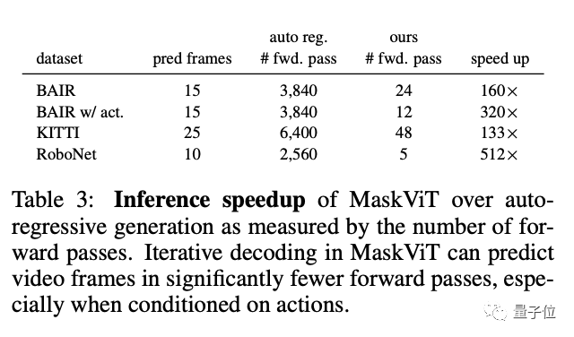
Lifeifei's team applied vit to the robot, increased the maximum speed of planning reasoning by 512 times, and also cued hekaiming's Mae

Tencent Peking University's sparse large model training acceleration program het was selected into the VLDB of the international summit
![[Blue Bridge Cup training 100 questions] scratch distinguishing prime numbers and composite numbers Blue Bridge Cup scratch competition special prediction programming question intensive training simul](/img/26/c0c8a406ff4ffe0ae37d277f730bd0.png)
[Blue Bridge Cup training 100 questions] scratch distinguishing prime numbers and composite numbers Blue Bridge Cup scratch competition special prediction programming question intensive training simul
随机推荐
OpenSea上如何创建自己的NFT(Polygon)
手写数字体识别,用保存的模型跑自己的图片
R language plot visualization: plot visualizes the normalized histogram, adds the density curve KDE to the histogram, and uses geom at the bottom edge of the histogram_ Adding edge whisker graph with
11 introduction to CNN
stm32h7b0替代h750程序导致单片机挂掉无法烧录程序问题
Failed to upload hyperf framework using alicloud OSS
mha 切换(操作流程建议)
What is the process of switching C # read / write files from user mode to kernel mode?
11 cnn简介
长安链交易防重之布谷鸟过滤器
补齐短板-开源IM项目OpenIM关于初始化/登录/好友接口文档介绍
【时间复杂度和空间复杂度】
Oilfield exploration problems
牛客编程题--必刷101之动态规划(一文彻底了解动态规划)
NFT contract basic knowledge explanation
[207] several possible causes of Apache crash
Simple use of tensor
2 three modeling methods
Detailed explanation of cookies and sessions
TCP拥塞控制详解 | 1. 概述