10 Exploring Temporal Information for Dynamic Network Embedding 5
Abstract
In this paper, we propose a new method called DTINE Unsupervised deep learning model , The model explores time information , To further enhance the robustness of node representation in dynamic networks . In order to maintain the network topology , A time weight and sampling strategy are designed to extract features from neighbors . Apply the attention mechanism to RNN, To measure the contribution of historical information , Capture the evolution of the network .
Conclusion
This paper discusses the influence of introducing time information into network embedding . A new unsupervised model is proposed DTINE, The model keeps dynamic topology by extracting neighborhood features , And pass LSTM Layer learning network evolution . The future work : Introduce more information , Such as node labels and node attributes , Expressed as rich nodes , And run on a larger network . Besides , Apply graph convolution to the model , So as to learn more potential characteristics when aggregating information .
Figure and table

chart 1 Examples of dynamic graphs ,(a) Expressed as continuous time dynamic graph ,(b) Expressed as a from (a) Split snapshot set , Discrete time dynamic graph

chart 2:DTINE frame . We first extract features from our neighbors , And then through multiple LSTM Layer to explore the time information of dynamic network . Optimize learning parameters through node interaction .

surface 1 Dataset parameters

surface 2 stay \(t\) Time graph reconstruction comparison
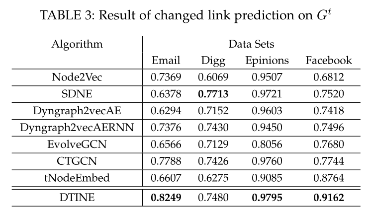
surface 3 stay \(t\) Link prediction comparison of time

surface 4 stay \(t+1\) Link prediction comparison of time
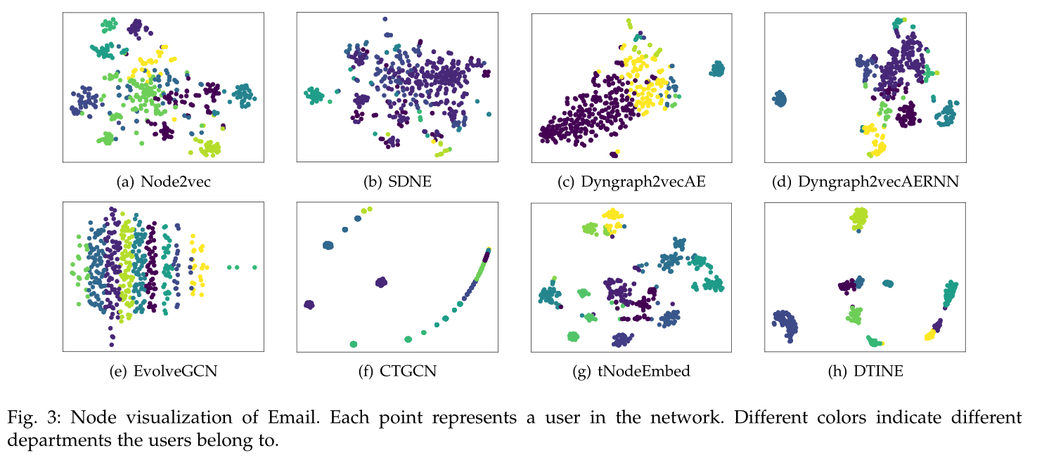
Figure 3 Data sets Email Node visualization of , Each node represents a user , Color represents user classification .

surface 5 The influence of temporal information on the model

chart 4 The impact of different embedded dimensions on each model and data set

chart 5 The impact of different snapshot numbers on each model and each dataset

chart 5 \(\beta_0\) The impact of different data sets on this model
Introduction
In the real world , The network is dynamic in nature , Its structure has evolved over time . There are two ways to describe dynamic networks , Pictured 1(a) Sum graph 1(b) Shown . The first method combines all the links into a large network , stay Continuous-time dynamic network embeddings Is called continuous time network , Each of these edges has a timestamp . The second method is to segment several snapshots of dynamic graph pairs . Each snapshot contains a small portion of the link . just as CTDNE As discussed in , Due to coarser aggregation granularity and interruption of edge flow , The latter method may result in information loss . Discrete time intervals also need to be carefully selected . Decomposing dynamic network into snapshots is an effective method to express the changes of network structure and properties . This method can easily capture the evolution process of the network . Pictured 1(b) Shown , stay t moment ,\(v_1\) Communicate with other users . hypothesis \(v_2、v_3、v_4\) Like sports , and \(v_5、v_6、v_7\) Like watching movies . They can be divided into different groups according to their interests . stay \(t + 1\) moment ,\(v_1\) Like and \(v_2\) Exercise together ,\(v_2\) Then I introduced him to some new friends . as time goes on , He was attracted by some movies , And turn your attention to the rest of the movie community , such as \(v_5, v_6, v_7\). The changing patterns of users can reflect how the network develops over time . Exploring this time information enables us to effectively discover users' social strategies , And predict links more accurately .
Previous work only considered structural information , Use static methods on each snapshot , Then align the embedded results across time steps . But when the network operates independently, it may have unstable consequences . Even if the network is similar , The result of embedding may be completely different , This makes it difficult to capture the process of change . Besides , These efforts cannot be extended to large networks , Because on each snapshot node2vec[28] and GCN[9] And other methods require a lot of parameter learning , Time consuming . Other methods generate time random walks to capture network evolution . However , This will also lead to the problem of spatial discontinuity mentioned above , If the changing parts of the network are large , Walking can be very complicated .
The contribution of this paper is as follows
A new method named DTINE The unsupervised approach to , Use dynamic topology to learn network representation .
Two special attention mechanisms are proposed for feature extraction and network training , Historical information can be further explored .
A large number of experimental results show that ,DTINE Significant improvements to several state-of-the-art baselines have been achieved .
Method
3 PROBLEM DEFINITION
Definition 1 (Dynamic network): Given a sequential network \(\mathcal{G}=<\mathcal{V,E,T}>\) , among V Is the set of all nodes ,E Is the set of all edges ,T Is a function that maps each edge to a timestamp .G It can be a directed graph or an undirected graph . Based on timestamps , The dynamic network will be split into a series of equally spaced snapshots \({G_1, G_2,…, G_T}\).\(T\) For the time step ,\(G^t=<V^t, E^t, A^t>\) It is expressed as a in time t A snapshot of the graph of .\(E^t\) Contains a fixed time interval \([t, t + τ]\) Inner edge . Be careful , stay \(E^t\) in , node \(v_i\) and \(v_j\) There may be multiple edges between . Will be in \(E^t\) The existence of multiple edges at the same node in is represented as \(A_{i j}^{t}=L^{t}(i, j)\), among \(L^{t}(i, j)\) Is the node \(v_i\) and \(v_j\) In time \(t\) Link frequency . This article assumes that the number of nodes for all snapshots remains the same . Invisible or deleted nodes \(i\) Will be treated as an isolated node , And make \(A^t[i,:] = 0\).
Definition 2 (Temporal network embedding): Suppose the last snapshot \(G^t\) It is a static network , The model aims to learn a mapping function \(f:v_i→ \mathbb{R}^d , d << N\) Make go through \(\{ G^1, G^2, ..., G^{t−1} \}\) After the snapshot training , node \(v\) There are appropriate embedded representations , among \(d\) The dimension represented for each node ,\(N\) Is the number of nodes . The goal of this article is to preserve structural information ( The nearest node has a similar representation ) And time information ( Nodes can explore potential relationships in the future ).
4 PROPOSED METHOD
The model consists of two parts
The first component is a graph based convolution network , It learns node representation by aggregating features from neighbors . The difference is , In the work of this paper , The weight of the edge will be updated with historical information .
The second component explores time attributes through snapshots . We're going to do it through LSTM The layer adds an attention mechanism to model the contribution of each snapshot .
DTINE The frame of is as shown in the figure 2 Shown . Extract the features obtained from the previous time step in each snapshot , These features will be concatenated and input into LSTM layer . The final node representation is based on specific rules from LSTM From the aggregation of hidden states .
4.1 Feature Initialization
In most networks , Connections between nodes are very sparse . This leads to a large number of zero elements in the adjacency matrix . Operate on the sparse matrix directly without any additional features , It may increase the complexity of time and space , And cause information redundancy in the model . So the author applies static algorithm to extract structural features when initializing features , such as node2vec.
4.2 Feature Extraction
For sequence diagram modeling , The author thinks that it is a snapshot of a graph at different times \(\{ G^1, G^2, ..., G^{t} \}\) Link change modeling in . Suppose that the evolution of the network can be seen as the change of the neighborhood of each node ( Added or deleted Links ), This is ultimately reflected in changes in information aggregation .
However , The same node may focus on different points in the snapshot . For example, in figure 1(b) in , stay \(t + 1\) moment ,\(v1\) And \(v_2\)、\(v_3\)、\(v_4\) Have the same interest in sports , The connection strength between them is higher than that of others . And then in \(t + 2\) When ,\(v_1\) I prefer to watch movies , and \(v_5\)、\(v_6\)、\(v_7\) Share his feelings , This leads to a greater weight between them . Be careful , stay \(v2\) There are no added or deleted links with its neighbors , But their weights have changed . therefore , If we want to model network evolution and capture time information , Should not treat every neighbor equally . let me put it another way , Each neighbor's contribution should be assessed , Instead of training the average aggregator to gather information .
In this paper , A new weight strategy is proposed , This strategy can estimate the link weights between nodes with the development of the network . among , Specific snapshots t Two connected nodes in \(i\) and \(j\) The strength function of can be expressed as :
among
In the equation (1) in , Considering the influence of structure and time .
The first term can be thought of as the source node \(i\) And target nodes \(j\) The strength of the structural connection between .\(D(i)\) Is the node \(i\) Degree ,\(D_\text{common}(i, j)\) Indicates in the snapshot \(i\) and \(j\) The number of common neighbors . Be careful , If two nodes have many common neighbors , Then they are similar to each other . If a node has a large degree , Will turn your attention to other nodes , The weight is small .
The second term considers the current and previous time steps , It can be regarded as a node \(i\) and \(j\) Time connection strength .\(λ_{i,j}\) Representation node \(i\) The node \(j\) The degree of influence .\(L(i, j)\) yes \([t−τ, t]\) Number of links between two nodes in , Because they may contact each other many times in a time interval .\(C(i, j)\) Representation node \(i\) And nodes \(j\) Number of previous snapshots with links .\(C(i, j)\) The value of should be in \(0\) To \(t\) Between . The strength of the time connection indicates , node \(i\) and \(j\) In time t The more previous connections , The greater the weight . say concretely , If one node remains connected to other nodes , Their relationship should be very stable , It leads to greater affinity between them .
In order to ensure the comparability of weight coefficients , It is recommended to use softmax Function to normalize the weight coefficient :
among \(\mathcal{N}(i)\) Express \(i\) Neighbors of . Adopt the attention mechanism similar to other models , utilize \(\alpha_{i, j}\) and 1 Skip neighbor extraction information . therefore , node \(i\) The influence of neighbors can be expressed as :
among
\(U^{t-1}(i)\) by \(i\) The representation in the previous snapshot
\(N (i)\) Express \(i\) Neighbors of .
Second order similarity is a very important measure , It can simulate the similarity between nodes , And keep the global structure . Therefore, information aggregation of two hop neighbors is introduced , There is no attention weight , Instead, we use the mean aggregation
among \(N^2(i)\) by \(i\) Of 2 Jump neighbor ,\(|N^2(i)|\) by 2 Jump the number of neighbors .
Here are the time smoothing assumptions : The author thinks that , In the real world , The changes of edges are smooth , let me put it another way , Only a few edges will be added or deleted in two consecutive time snapshots .
therefore , Embedding should change smoothly over time , This means that if a node and its neighborhood are similar in two snapshots , Then its representation should remain similar .
Suppose we don't model smooth changes , Due to the loss of regularity between node representations , It may be difficult to capture the evolution of the network . To achieve this goal , We will be the first to t Nodes in snapshots i Expressed as :
among \(β_0 + β_1 = 1\), And \(β_0 > β_1\), These two coefficients are used to measure the first-order and second-order adjacent contributions . The above formula ensures that the node representation changes smoothly , Because over time , Their transformations in the embedded space are linear ( Incremental addition and subtraction ).
4.3 Sampling Strategy
With the expansion of the network , The number of neighbors will also increase , Causes more memory and computation to be consumed when aggregating information . So a method of effectively extracting neighbor information and removing redundant information is proposed . among , node \(i\) Neighbors of \(j\) The probability of being sampled is expressed as
among \(\varphi_{0} \in\left[0,1-\frac{1}{[\mathcal{N}(i)}\right], \varphi_{1} \in\left[0, \frac{1}{\mid \mathcal{N}(i)}\right]\), This sampling strategy strengthens that the nodes connected by the newly updated edges should get more weight
In the 4.2 In the festival , This strategy will sample the neighbor set , And when aggregating information \(\mathcal{N}_\text{sample}(i)\) Replace \(\mathcal{N} (i)\). about 2 Jump neighbor \(\mathcal{N}^2(i)\), We only use random sampling .
4.4 Temporal Node Embedding
The author explains why LSTM:
Suppose we aggregate the information of each node in all snapshots . The key point is how to combine these discrete representations and get the final embedded results , Because node interactions are independent between snapshots . By machinetranslation 、 Text classification, etc , In natural language processing , Each node in the timeline can be regarded as a word in the sentence .
therefore , have access to LSTM[42] Learn the hidden layer node representation . take LSTM The layer is defined as follows
\(h_t(i)\) Contains all the information under the time step , However , Each snapshot has a different contribution to the last node representation , namely , Events in the previous time step can affect the current representation to varying degrees .
For example, figure 1(b) in ,\(v_1\) At first, I tend to communicate with people who like sports . as time goes on , He was attracted to other things , Such as watching movies and drawing pictures . But when he returned to his interest in sports , Time is \(n + t\), We can find many friends in time \(t\) Reappear on his communication list . therefore , The first \(t\) The neighborhood information of snapshots has the most significant impact on the current node representation . Its mathematical expression is
In order to effectively simulate the contribution of historical information , We are LSTM Attention mechanism is added to the network . set up \(H(i)\) yes \([h_0(i), h_1(i),…,h_T (i)]\),\(H(i) ∈ R^{T ×d}\), In style \(T\) Is the number of snapshots ,\(d\) by LSTM Hidden dimension of the layer . There is the following formula
among
\(w_{1} \in \mathbb{R}^{1 \times d}, w_{2} \in \mathbb{R}^{T \times d}\) For learning parameters , Respectively for \(H(i)\) and \(h_T (i)\) convert .
\(h^s(i) \in \mathbb{R}^{1 \times d}\) For the node \(i\) In the final snapshot \(G^t\) In means , It can save time information .
The goal of the loss is to embed the node with the highest constraint similarity into the closest potential space . meanwhile , Discrete or distant nodes will be penalized . The losses are as follows :
among
\(N_{walk}(i)\) Is a random walk node \(i\) A collection of nearby nodes .
\(p_n\) Is a negative sampling distribution ,\(Q\) Is the number of negative nodes sampled
\(\nu\) Is the attenuation coefficient ,\(W\) Is the learning parameter of the model . The weight attenuation term can prevent over fitting in the training stage .
\(h^s (i),h^s (j)\) To calculate the inner product of the node's indirect proximity . The random gradient descent method is used to optimize the loss function .
The calculation process of the model is shown in the algorithm 1.
The first 2-9 Behavior extracts features from neighborhood , And ensure that the nodes embedded in the time step change smoothly .
The first 10-14 Row iteration \(G^T\) Node training LSTM, Capture network evolution .

Experiment
5 EXPERIMENTS
5.1 Data Sets
The data set and its parameters are shown in table 1
5.2 Baselines
Node2Vec
SDNE
Dyngraph2vecAE ,Dyngraph2vecAERNN
EvolveGCN
CTGCN
tNodeEmbed
5.3 Experimental Setup
use AUC As an indicator ,
The embedding dimension is set to 128
Weight attenuation coefficient \(\nu\) by 0.001
about Facebookand Digg, The learning rate is 0.001, And in the Email The secondary school attendance rate will be 0.0003. Set the number of snapshots to 12 individual .
5.4 Experimental Results
5.4.1 Link Prediction
Link reconstruction See table 2
Changed link prediction See table 3 surface 4
Removing temporal part See table 5
5.5 Parameter Sensitivity
Embedding dimension See the picture 4
Number of snapshots See the picture 5
Summary
In this article, I learned to use node2vec To initialize the graph embedding , After reading the whole article, the conclusion is DTDG Use time smoothing to simulate as much as possible CTDG, Then we use the class GCN Information aggregation of , Random sampling is used to reduce the amount of calculation , Attention weight is used to control the influence of neighbors , use LSTM Save timing information , On the whole, I don't see anything new , Another article on building blocks