当前位置:网站首页>Machine learning practice notes
Machine learning practice notes
2022-07-24 14:20:00 【Strong fight】
Chapter one — End to end machine learning projects
Common operations of data preprocessing :
Set coordinate axis labels and scales in the subgraph .set_xlabel .set_xticks
– Data mapping —>data[col_name == Original value ,col_name]= Mapping values
– Get the list of column names —>col_names = data.columns.tolist()
– Remove some irrelevant columns —>todrop=[’’,’’] data.drop(todrop,axis=1)
– There is a large difference between the two equally important columns —> Standardization
– Select some qualified rows , First, traverse and save the qualified indexes in the list , then data.loc[list,:]
Download data
Write a function to get data
def fetch_housing_data(housing_url=url,housing_path=path):
    if not os.path.isdir(housing_path):
        os.makedirs(housing_path)
    tgz_path = os.path.join(housing_path,"housing.tgz")
    urllib.request.urlretrieve(housing_url, tgz_path)
    housing_tgz = tarfile.open(tgz_path)
    housing_tgz.extractall(path=housing_path)
    housing_tgz.close()
Write a function to load data
import pandas
def load_housing_data(housing_path=HOUSING_PATH):
    csv_path = os.path.join(housing_path,"housing.csv")
    return pd.read_csv(csv_path)
Watch the big picture
Quick view of data structure
info() You can quickly get a simple description of the dataset , Especially the total number , The type of each property and the number of non null values
value_counts() Check how many categories exist , Each category can display a summary of numeric attributes
describe() Displays a summary of numeric properties
Called on the entire dataset hist() Method , Draw a histogram of each attribute
example :
import matplotlib.pyplot as plt
      housing.hist(bins=50,figsize(20,15))
      plt.show()
Create test set
( Pure random sampling method )
from sklearn.model_selection import train_test_split
predictors = ["col1", "col2"]
x_train, x_test, y_train, y_test = train_test_split(data[predictors], data["target"], test_size=0.4, random_state=0)
( Stratified sampling )
col Columns are hierarchical based columns
from sklearn.model_selection import StratifiedShuffleSplit
split = StratiffiedShuffleSplit(n_splits=1, test_size=0.2, random_state=42)
for train_index,test_index in split.split(data,data["col"]):
    start_train_set = data.loc[train_index]
    start_test_set = data.loc[test_index]
To delete the same attribute of training set and test set :
for set in (start_train_set, start_test_set):
    set.drop(["clo"], axis=1, inplace=True)
Data exploration and Visualization
① Geographic Data Visualization :
housing.plot(kind="scatter", x="longtitude", y="latitude", alpha=xxx
                    s=housing["population"]/100,label="population"
                    c="median_house_value",cmap=plt.get_cmap("jet"),colorbar=True)
                    # It can also depict  X And Y The correlation between attributes
                    import matplotlib.pyplot as plt
                    plt.show()
② Looking for relevance :
(col Column correlation with other columns )
corr_matrix = data.corr()
corr_matrix[“col”].sort_values(ascendsing=False)
Pearson correlation coefficient : The closer the 1, Indicates that there is a stronger positive correlation , The closer the -1, Indicates that there is a stronger negative correlation
Plot the correlation of each numeric attribute with respect to other numeric attributes .
from pandas.tools.plotting import scatter_matrix
attributes = ["col1","col2","col3","col4"]
scatter_matrix(housing[attribute],figsize=(12,8))
Experiment with combinations of different attributes
example :housing[“rooms_per_household”] = housing[“total_rooms”]/housing[“households”]
③ Data preparation :
data = train_set.drop(“col”, axis=1)
label = train_set[“col”].copy
drop() A copy of the data will be created , But it doesn't affect data
Data cleaning :
col Some values of column attributes are missing , terms of settlement :
- Discard the corresponding value :data.dropna(subset=[“col”])
- Discard this attribute :data.drop(“col”,axis=1)
- Set the missing value to a value :data[“col”].fillna(median)
Handling missing values :
from sklearn.preprocessing import Imputer
imputer = Imputer(strategy=“median”)
Use fit() Methods will imputer Instance adaptation to training set :
imputer.fit(housing_num)
here imputer Only the median value of each attribute is calculated , And store the result in its instance variable statistics_
X=imputer.transform(housing_num)
Handle text and classification properties
skikit-learn It provides a converter for such tasks LabelEncoder:
from sklearn.preprocessing import LabelEncoder
encoder = LabelEncoder()
housing_cat = housing["ocean_proximity"]
housing_cat_encoded = encoder.fit_transform(housing_cat)
housing_cat_encoded
The resulting problems : Machine learning algorithms assume that two numbers that are close to each other are more similar than two numbers that are far away
To solve this problem , A common solution is to create a binary attribute for each category , Hot coding alone
Scikit-learn Provides a OneHotEncoder Encoder , The integer classification value can be converted into a single heat vector
from sklearn.preprocessing import OneHotEncoder
encoder = OneHotEncoder()
housing_cat_1hot = encoder.fit_transform(housing_cat_encoded.reshape(-1,1))
The output here is a Scipy sparse matrix
Use LabelBinarizer Class can perform two transformations at once ( Convert from text category to integer category , Then it is converted from integer category to independent heat vector )
from sklearn.preprocessing import LabelBinarizer
encoder = LabelBinarizer()
housing_cat_1hot = encoder.fit_transform(housing_cat)
By sending sparse_output=True to LabelBinarizer Constructors , We can get the sparse matrix
Calculation RMSE
from sklearn.metrics import mean_squared_error
housing_predictions = lin_reg.predict(housing_prepared)
lin_mse = mean_squared_error(housing_labels, housing_predictions)
lin_rmse = np.sqrt(lin_mse)
Use cross validation to better evaluate
from sklearn.model_selection import cross_val_score
scores = cross_val_score(tree_reg,housing_prepared,housing_labels,scoring="neg_mean_squared_error",cv=10)
rmse_scores = np.sqrt(-scores)
Random forests
from sklearn.ensemble import RandomForestRegressor
forest_reg = RandomForestRegressor()
forest_reg.fit(housing_prepared,housing_labels)
Fine tune the model
The grid search
It can be used scikit-learn Of GridSearchCV To explore
from sklearn.model_selection import GridSearchCV
param_grid = [
   {'n_estimators':[3,10,30],'max_features':[2,4,6,8]},
   {'bootstrap':[False],'n_estimators':[3,10],'max_features':[2,3,4]},
    ]
  forest_reg = RandomForestRegressor()
  grid_search = GridSearchCV(forest_reg, param_grid, cv=5, scoring='neg_mean_squared_error')
  grid_search.fit(housing_prepared,housing_labels)
param_grid tell scikit-learn First evaluate the first dict in n_estimator and max_features All of the 34=12 A super parameter combination
next Try the second dict Zhongchao parameter values all 23=6 Combinations of , But this time the hyperparameter bootstrap I need to set to False instead of True
Optimal parameter combination :grid_search.best_params_
Random search
When the search range of the super parameter is large , Usually... Is preferred RandomizedSearchCV
If you run a random search 1000 An iterative , We will explore the... Of each super parameter 1000 Different values .
Analyze the best model and its mistakes
randomforestregressor You can point out the relative importance of each attribute
feature_importances = grid_search.best_estimator_.feature_importances_
Display these importance scores next to the corresponding attribute name :
sorted( zip(feature_importances,attributes),reverse=True )
Evaluate the system through the test set
final_model = grid_search.best_estimator_

x_test = start_test_set.drop("median_house_value",axis=1)
y_test = start_test_set["median_house_value"].copy()
x_test_prepared = full_pipeline.transform(x_test)
final_predictions = final_model.predict(x_test_prepared)

final_mse = mean_squared_error(y_test,final_predictions)
final_rmse = np.sqrt(final_mse)
Two . classification
MNIST Data sets , Each picture is marked with the number it represents .
x,y = minst[“data”],minst[“target”]
x.shape
y.shape
Each picture has 784 Features . Because the picture is 28*28 Pixels , Each feature represents the intensity of a pixel , from 0( white ) To 255( black )
display picture
import matplotlib
import matplotlib.pyplot as plt
some_digit = X[36000]
some_digit_image = some_digit.reshape(28,28)
plt.imshow(some_digit_image, cmap = matplotlib.cm.binary,interpolation="nearest")
plt.axis("off")
plt.show()
Training set data shuffle
x_train,x_test,y_train,y_test = X[:60000],X[60000:],Y[:60000],Y[60000:]
import numpy as np
shuffle_index = np.random.permutation(60000)
x_train,y_train =x_train[shuffle_index],y_train[shuffle_index]
Train a binary classifier
First create an objective vector for this classification task :
y_train_5 = (y_train == 5)
y_test_5 = (y_test == 5)
Training :
from sklearn.linear_model import SGDClassifier
sgd_clf = SGDClassifier(random_state=42)
sgd_clf.fit(x_train,y_train_5)
sgd_clf.predict([some_digit])
Implement cross validation :
from sklearn.model_selection import StratifiedKFold
from sklearn.base import clone
skfolds = StratifiedKFold(n_split=3, random_state=42)
for train_index,test_index in skfolds.split(x_train,y_train_5):
clone_clf = clone(sgd_clf)
x_train_folds = x_train[train_index]
y_train_folds = (y_train_5[train_index])
x_test_fold = x_train[test_index]
y_test_fold = (y_train_5[test_index])
clone_clf.fit(x_train_folds,y_train_folds)
y_pred = clone_clf.predict(x_test_fold)
n_correct = sum(y_pred == y_test_fold)
print(n_correct / len(y_pred)
Each fold is StratifiedKFold Perform stratified sampling to generate , The proportion symbol of each class it contains is the overall proportion .
Confusion matrix
A better way to evaluate the performance of classifiers is the confusion matrix
from sklearn.model_selection import cross_val_predict
y_train_pred = cross_val_predict(sgd_clf,x_train,y_train_5,cv=3)
And cross_val_score() The function is the same ,cross_val_predict() The function also performs K-fold Cross validation , But it doesn't return the evaluation score , But each
Folded prediction .
from sklearn.metrics import confusion_matrix # Use this function to get the confusion matrix
confusion_matrix( Target categories , Forecast category )
The rows in the confusion matrix represent the actual categories , List forecast categories .
A perfect classifier has only true classes and true negative classes , So its confusion matrix will only have non-zero values on its diagonal
precision :TP/(TP+FP) How many predictions are accurate
Recall rate =TP/(TP+FN)
scikit-learn It provides functions for calculating various classifier indicators , Accuracy and recall rate are also one of them
from sklearn.metrics import precision_score,recall_score
precison_score(y_train,y_pred)
recall_score(y_train,y_train_pred)
Combine precision and recall into a single index , be called F1 fraction ,F1 Is the harmonic average of accuracy and recall
To calculate F1 fraction , Just call f1_score()
from sklearn.metrics import f1_score
In some cases , More concerned about accuracy , In other cases , More concerned about recall rate
Multi label classification
Produce multiple categories for each instance , such as : Is a big number , It's odd again
from sklearn.neighbors import KNeightborsClassifier
y_train_large = (y_train >= 7)
y_train_odd = (y_train %2 ==1)
y_multilabel = np.c_[y_train_large,y_train_odd]
knn_clf = KNeighborsClassifier()
knn_clf.fit(X_train,y_multilabel)
Multi output classification
Use Numpy Of randint() Function is MNIST The pixel intensity of the picture increases noise . The goal is to restore the image to the original image :
noise = rnd.randint( 0,100,(len(x_train),784) )
noise = rnd.randint( 0,100,(len(x_test),784) )
x_train_mod = x_train + noise
x_test_mod = x_test +noise
knn_clf.fit(x_train_mod, y_train_mod)
clean_digit = knn_clf.predict( [x_test_mod[some_index]] )
plot_digit(clean_dight)
边栏推荐
- The sliding window of Li Kou "step by step" (209. The smallest sub array, 904. Fruit baskets)
- Rasa 3.x 学习系列-Rasa [3.2.4] - 2022-07-21 新版本发布
- Csp2021 T1 corridor bridge distribution
- Attributeerror: module 'distutils' has no attribute' version error resolution
- 字符串——剑指 Offer 58 - II. 左旋转字符串
- Atcoder beginer contest 261 f / / tree array
- MySQL community download address
- 【机器学习】之 主成分分析PCA
- REST风格
- C operator priority memory formula
猜你喜欢

Uni app background audio will not be played after the screen is turned off or returned to the desktop

Regular expression and bypass cases
![Rasa 3.x 学习系列-Rasa [3.2.3] - 2022-07-18 新版本发布](/img/fd/c7bff1ce199e8b600761d77828c674.png)
Rasa 3.x 学习系列-Rasa [3.2.3] - 2022-07-18 新版本发布
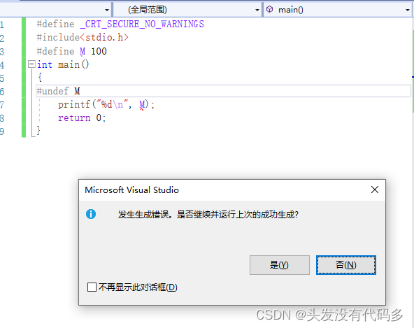
C language -- program environment and preprocessing

Solve the problem of repeated clicking of button uibutton

Dameng real-time active and standby cluster construction

Attributeerror: module 'distutils' has no attribute' version error resolution
Solve the problem that the ARR containsobject method returns no every time

Number of bytes occupied by variables of type char short int in memory
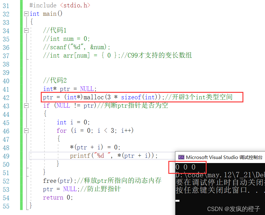
【C语言笔记分享】——动态内存管理malloc、free、calloc、realloc、柔性数组
随机推荐
Grpc middleware implements grpc call retry
Matlab program for natural gas flow calculation
Unity pedestrians walk randomly without collision
MySQL community download address
REST风格
2022年IAA行业品类发展洞察系列报告·第二期
字符串——28. 实现 strStr()
C# unsafe 非托管对象指针转换
栈与队列——20. 有效的括号
mysql
交换
TypeError: 'str' object does not support item assignment
Summary of week 22-07-23
Nmap security testing tool tutorial
字符串——剑指 Offer 58 - II. 左旋转字符串
JS judge whether it is an integer
Centos7安装达梦单机数据库
threw exception [Circular view path [index]: would dispatch back to the current handler URL [/index]
[oauth2] II. Known changes in oauth2.1
Summary of Baimian machine learning