当前位置:网站首页>Fill the pit for repvgg? In fact, it is the repoptimizer open source of repvgg2
Fill the pit for repvgg? In fact, it is the repoptimizer open source of repvgg2
2022-06-23 09:39:00 【Zhiyuan community】
In the design of neural network structure , We often introduce some prior knowledge , such as ResNet Residual structure of . However, we still use the conventional optimizer to train the network . In this work , We propose to use prior information to modify gradient values , It is called gradient reparameterization , The corresponding optimizer is called RepOptimizer. We focus on VGG The straight cylinder model of , Train to get RepOptVGG Model , He has high training efficiency , Simple and direct structure and extremely fast reasoning speed .

Thesis link :https://arxiv.org/abs/2205.15242
Official warehouse :https://github.com/DingXiaoH/RepOptimizers
And RepVGG The difference between
- RepVGG A structural prior is added ( Such as 1x1,identity Branch ), And use the regular optimizer to train . and RepOptVGG It is Add this prior knowledge to the optimizer implementation
- Even though RepVGG In the reasoning stage, the branches can be fused , Become a straight tube model . however There are many branches in the training process , Need more memory and training time . and RepOptVGG But really - Straight cylinder model , From the training process is a VGG structure
- We do this by customizing the optimizer , The equivalent transformation of structural reparameterization and gradient reparameterization is realized , This transformation is universal , It can be extended to more models

Introducing structural prior knowledge into the optimizer
We noticed a phenomenon , In special circumstances , Each branch contains a linearly trainable parameter , Add a constant scaling value , As long as the scaling value is set reasonably , The performance of the model will still be very high . We call this network block Constant-Scale Linear Addition(CSLA) Let's start with a simple CSLA Start with examples , Consider an input , after 2 A convolution branch + Linear scaling , And added to an output , We consider equivalent transformation into a branch , The equivalent transformation corresponds to 2 A rule :
Initialization rules
The weight of fusion shall be :

update rule
For the weight after fusion , The update rule is :

For this part of the formula, please refer to appendix A in , There is a detailed derivation. A simple example code is :
import torchimport numpy as npnp.random.seed(0)np_x = np.random.randn(1, 1, 5, 5).astype(np.float32)np_w1 = np.random.randn(1, 1, 3, 3).astype(np.float32)np_w2 = np.random.randn(1, 1, 3, 3).astype(np.float32)alpha1 = 1.0alpha2 = 1.0lr = 0.1conv1 = torch.nn.Conv2d(1, 1, kernel_size=3, padding=1, bias=False)conv2 = torch.nn.Conv2d(1, 1, kernel_size=3, padding=1, bias=False)conv1.weight.data = torch.nn.Parameter(torch.tensor(np_w1))conv2.weight.data = torch.nn.Parameter(torch.tensor(np_w2))torch_x = torch.tensor(np_x, requires_grad=True)out = alpha1 * conv1(torch_x) + alpha2 * conv2(torch_x)loss = out.sum()loss.backward()torch_w1_updated = conv1.weight.detach().numpy() - conv1.weight.grad.numpy() * lrtorch_w2_updated = conv2.weight.detach().numpy() - conv2.weight.grad.numpy() * lrprint(torch_w1_updated + torch_w2_updated)import torchimport numpy as npnp.random.seed(0)np_x = np.random.randn(1, 1, 5, 5).astype(np.float32)np_w1 = np.random.randn(1, 1, 3, 3).astype(np.float32)np_w2 = np.random.randn(1, 1, 3, 3).astype(np.float32)alpha1 = 1.0alpha2 = 1.0lr = 0.1fused_conv = torch.nn.Conv2d(1, 1, kernel_size=3, padding=1, bias=False)fused_conv.weight.data = torch.nn.Parameter(torch.tensor(alpha1 * np_w1 + alpha2 * np_w2))torch_x = torch.tensor(np_x, requires_grad=True)out = fused_conv(torch_x)loss = out.sum()loss.backward()torch_fused_w_updated = fused_conv.weight.detach().numpy() - (alpha1**2 + alpha2**2) * fused_conv.weight.grad.numpy() * lrprint(torch_fused_w_updated)stay RepOptVGG in , Corresponding CSLA Blocks are RepVGG In the block 3x3 Convolution ,1x1 Convolution ,bn The layer is replaced by With learnable scaling parameters 3x3 Convolution ,1x1 Convolution Further expand to multi branch , hypothesis s,t Namely 3x3 Convolution ,1x1 Scaling coefficient of convolution , Then the corresponding update rule is :

The first formula corresponds to the input channel == Output channel , There is a total of 3 Branches , Namely identity,conv3x3, conv1x1 The second formula corresponds to the input channel != Output channel , At this time only conv3x3, conv1x1 The third formula of the two branches corresponds to other situations. It should be noted that CSLA No, BN This nonlinear operator during training (training-time nonlinearity), There is no non sequency (non sequential) Trainable parameter .
边栏推荐
- Redis学习笔记—redis-benchmark详解
- #gStore-weekly | gStore源码解析(四):安全机制之黑白名单配置解析
- 2022 Gdevops全球敏捷运维峰会-广州站精华回放(附ppt下载)
- 【CTF】bjdctf_ 2020_ babyrop
- 太阳塔科技招聘PostgreSQL数据库工程师
- 【CTF】 2018_ rop
- ARM中常见的英文解释
- Chain representation and implementation of linklist ---- linear structure
- The usage of lambda of C
- 启明星辰华典大数据量子安全创新实验室揭牌,发布两款黑科技产品
猜你喜欢
![[geek Challenge 2019] hardsql](/img/73/ebfb410296b8e950c9ac0cf00adc17.png)
[geek Challenge 2019] hardsql
![[GXYCTF2019]BabySQli](/img/51/a866a170dd6c0160ce98d553333624.png)
[GXYCTF2019]BabySQli

学习SCI论文绘制技巧(E)

Go 单元测试

Pizza ordering design - simple factory model

使用base64,展示图片
Redis learning notes pipeline
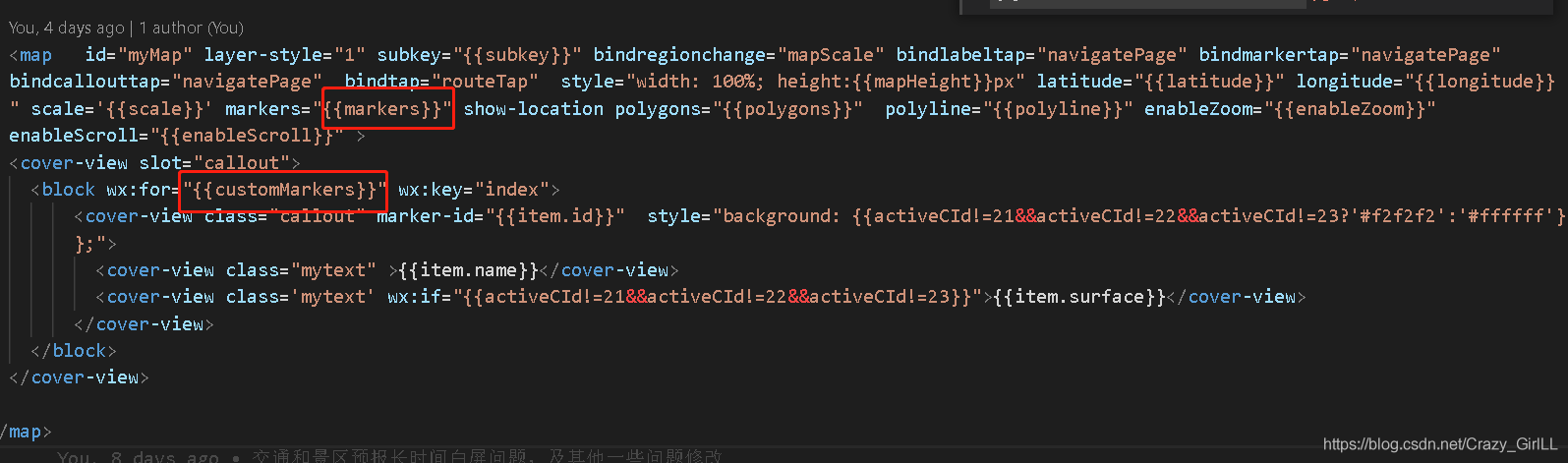
Wechat applet: click the button to switch frequently, overlap the custom markers, but the value does not change

swagger UI :%E2%80%8B

Zone d'entrée du formulaire ionic5 et boutons radio

随机推荐
Redis学习笔记—Pipeline
ionic5表单输入框和单选按钮
Leetcode topic analysis contains duplicate III
Jog sport mode
Learn SCI thesis drawing skills (f)
swagger UI :%E2%80%8B
Jump game of leetcode topic analysis
安装typescript环境并开启VSCode自动监视编译ts文件为js文件
Redis learning notes - redis cli explanation
Redis学习笔记—数据类型:集合(set)
我被提拔了,怎么和原来平级的同事相处?
UEFI 源码学习4.1 - PciHostBridgeDxe
Redis学习笔记—数据类型:字符串(string)
The usage of lambda of C
Redis学习笔记—地理信息定位(GEO)
Common English explanations in arm
Opening, creating and storing files
分布式锁的三种实现方式
[GXYCTF2019]BabyUpload
高性能算力中心 — NVMe/NVMe-oF — NVMe-oF Overview