当前位置:网站首页>Machine learning (Zhou Zhihua) Chapter 4 notes on learning experience of decision tree
Machine learning (Zhou Zhihua) Chapter 4 notes on learning experience of decision tree
2022-07-24 05:52:00 【Ml -- xiaoxiaobai】
The first 4 Chapter Decision tree The learning
The basic flow
It is mainly a recursive process
def TreeGenerate(D, A): # D For the sample set / list ,A For Attribute Collection
     Generate the nodes node
    if D  The samples in belong to the same class C:
        node Marked as C Leaf like node
        return
    if A  For an empty set ( That is, all attributes have been used up ) or D The sample is in A Same value as above :
         take node As leaf nodes , Marked as D The class with the largest number of samples
        return
     from A Choose the best attribute to divide attributes a_best
    for a in a_best The value of :
         from node Generate a branch point , Make D_divided by D In the a_best The property value is a A sample set of
        if D_divided is empty:
             This branch node becomes a leaf node , use D The class tag with the most samples in the class ( namely , When predicting a
             Sample time , The value of this property is a when , another use D Estimated by the largest number of categories , Obedience in the book
             A priori distribution of categories of parent nodes ).
            return
        else:
             The branch node is TreeGenetate(D_divided, A)
Divide and choose
Information gain (information gain)
Information entropy (information entropy)
Measure the probability of random variables “ Degree of confusion ” Of , The entropy mentioned in high school chemistry is a little different , This is very intuitive to understand with physical entropy , The larger the entropy, the more “ confusion ” The more “ Random ” The more ” disorder ”, The smaller the entropy, the more “ Orderly “ The more ” neat “. Formula for :
Ent ( D ) = − ∑ k = 1 ∣ Y ∣ p k log 2 p k \operatorname{Ent}(D)=-\sum_{k=1}^{|\mathcal{Y}|} p_{k} \log _{2} p_{k} Ent(D)=−k=1∑∣Y∣pklog2pk
commonly code Use directly e As the base number, don't 2.
Conditional entropy
Here, it is essentially understood as weighted information entropy , The formula is very intuitive :
∣ D v ∣ ∣ D ∣ Ent ( D v ) \frac{\left|D^{v}\right|}{|D|} \operatorname{Ent}\left(D^{v}\right) ∣D∣∣Dv∣Ent(Dv)
among D v D^{v} Dv From D D D Subset divided in ( Take a known “ Conditions ”).
So we can get the expression of information gain :
Gain ( D , a ) = Ent ( D ) − ∑ v = 1 V ∣ D v ∣ ∣ D ∣ Ent ( D v ) \operatorname{Gain}(D, a)=\operatorname{Ent}(D)-\sum_{v=1}^{V} \frac{\left|D^{v}\right|}{|D|} \operatorname{Ent}\left(D^{v}\right) Gain(D,a)=Ent(D)−v=1∑V∣D∣∣Dv∣Ent(Dv)
That is, subtract the divided conditional entropy from the undivided information entropy / Weighted information entropy , It is also intuitive , If the gap is bigger , It shows that the classification after classification is more “ Orderly ” Of course, it's the result we want . This is also ID3 The idea of Algorithm (Iterative Dichotomiser, Iterative two classifier ).
Gain rate (gain ratio)
ID3 One disadvantage of this information gain idea used by the algorithm is , When the attribute value increases , The resulting conditional entropy tends to become smaller ( The more classes , Naturally, each classification will be more tidy intuitively ), In extreme cases, each attribute value in the book corresponds to a sample , The conditional entropy is 0 了 , The information gain is the current maximum , But this situation obviously cannot be generalized well . So in order to balance , Balance the entropy increase caused by the increase of classification number ( Multi class itself is also a kind of disorder ), Therefore, we can use the entropy increase caused by the division itself to reduce the information gain , Formula for :
Gain ratio ( D , a ) = Gain ( D , a ) IV ( a ) \operatorname{Gain} \operatorname{ratio}(D, a)=\frac{\operatorname{Gain}(D, a)}{\operatorname{IV}(a)} Gainratio(D,a)=IV(a)Gain(D,a)
among ,
IV ( a ) = − ∑ v = 1 V ∣ D v ∣ ∣ D ∣ log 2 ∣ D v ∣ ∣ D ∣ \operatorname{IV}(a)=-\sum_{v=1}^{V} \frac{\left|D^{v}\right|}{|D|} \log _{2} \frac{\left|D^{v}\right|}{|D|} IV(a)=−v=1∑V∣D∣∣Dv∣log2∣D∣∣Dv∣
be called a The intrinsic value of (intrinsic value), In fact, according to A Entropy increase caused by set partition , Obviously, the more divisions, the more entropy increases , So as to balance the increase of information gain . Therefore, the gain rate has a certain preference for attributes with few values as partition attributes .
gini index (Gini index)
Define to take two samples randomly from the data set , The probability of not belonging to the same class is Gini value :
Gini ( D ) = ∑ k = 1 ∣ Y ∣ ∑ k ′ ≠ k p k p k ′ = 1 − ∑ k = 1 ∣ Y ∣ p k 2 \begin{aligned} \operatorname{Gini}(D) &=\sum_{k=1}^{|\mathcal{Y}|} \sum_{k^{\prime} \neq k} p_{k} p_{k^{\prime}} \\ &=1-\sum_{k=1}^{|\mathcal{Y}|} p_{k}^{2} \end{aligned} Gini(D)=k=1∑∣Y∣k′=k∑pkpk′=1−k=1∑∣Y∣pk2
Intuitively , If the purity of the data set is large , that Gini value The smaller it is .
Corresponding to information entropy and conditional entropy , Gini value is similar to Gini index “ weighting ” Relationship , gini index Defined as :
Gini_index ( D , a ) = ∑ v = 1 V ∣ D v ∣ ∣ D ∣ Gini ( D v ) \operatorname{ Gini\_index }(D, a)=\sum_{v=1}^{V} \frac{\left|D^{v}\right|}{|D|} \operatorname{Gini}\left(D^{v}\right) Gini_index(D,a)=v=1∑V∣D∣∣Dv∣Gini(Dv)
So the smaller Gini index , It means that the division purity is higher , This is a CART(Classification and Regression Tree) The idea of the algorithm .
Pruning (pruning)
To solve over fitting , Reduce the generation of too many leaf nodes , Control tree “ depth ”.
pre-pruning (prepruning)
In the process of generating nodes , Use the verification set to measure the generalization ability before and after node partition / Accuracy rate , Thus, the accuracy after division / Nodes with reduced generalization ability are divided into leaf nodes .
Pre pruning also has some problems , It cannot guarantee whether the reduction of generalization ability after the partition of a node is temporary , such as , After its division, if you continue to divide, you may achieve a lower error rate , Therefore, pre pruning has the risk of under fitting .
After pruning (postpruning)
Mr. A becomes a complete decision tree , Then investigate the intermediate nodes with leaf nodes from bottom to top , Check to remove the leaf nodes , After itself as a leaf node , Whether the correctness of the verification set is improved , If yes, prune .
Generally, the risk of under fitting after pruning is small , But the time cost of training is greater than the decision tree generation itself and pre pruning .
Continuous and missing values
Processing of continuous values
In fact, it is in the generation process of regression tree , Selection of dividing points , The book says, for example n Attributes , Then there are n-1 Points of division , Not necessarily , It's quite possible to add one , That is, all of them are transformed into one class . In this way, information gain can be avoided in practice , And heuristic learning , For example, those greater than a certain partition are positive classes , Less than is negative , Or less than is positive , Greater than is negative , Then find the optimal partition point according to the minimum error rate and take the inequality sign of greater or less ( See the code you wrote before ).
Processing of missing values
For the missing value, the book introduces C4.5 Processing method of algorithm , The basic idea can be summarized as , When selecting partition attributes , According to the weighted proportion of non missing samples in the total samples , weighting ( Calculated from a subset of samples without missing attribute values ) Information gain , So as to balance the difference of information gain of different attributes caused by different sample numbers ; After selecting the best attribute , When dividing sub nodes , For samples with missing attributes , Distribution of the number of samples divided according to no missing samples , The number of samples is weighted and divided into each node ( Equivalent to, for example, will 0.1 Samples are distributed to a child node ), This quantity will be retained or re divided in the future “ weighting ”( In addition, when the partition attribute is also missing a value ).
In particular , Definition :
ρ = ∑ x ∈ D ~ w x ∑ x ∈ D w x \rho=\frac{\sum_{\boldsymbol{x} \in \tilde{D}} w_{\boldsymbol{x}}}{\sum_{\boldsymbol{x} \in D} w_{\boldsymbol{x}}} ρ=∑x∈Dwx∑x∈D~wx
p ~ k = ∑ x ∈ D ~ k w x ∑ x ∈ D ~ w x ( 1 ⩽ k ⩽ ∣ Y ∣ ) \tilde{p}_{k}=\frac{\sum_{\boldsymbol{x} \in \tilde{D}_{k}} w_{\boldsymbol{x}}}{\sum_{\boldsymbol{x} \in \tilde{D}} w_{\boldsymbol{x}}} \quad(1 \leqslant k \leqslant|\mathcal{Y}|) p~k=∑x∈D~wx∑x∈D~kwx(1⩽k⩽∣Y∣)
r ~ v = ∑ x ∈ D ~ v w x ∑ x ∈ D ~ w x ( 1 ⩽ v ⩽ V ) \tilde{r}_{v}=\frac{\sum_{\boldsymbol{x} \in \tilde{D}^{v}} w_{\boldsymbol{x}}}{\sum_{\boldsymbol{x} \in \tilde{D}} w_{\boldsymbol{x}}} \quad(1 \leqslant v \leqslant V) r~v=∑x∈D~wx∑x∈D~vwx(1⩽v⩽V)
Among them w x w_{\boldsymbol{x}} wx Quantity weight , At first, it was 1, Represents the number of each sample itself , When there is a missing value and it is divided according to the missing attribute , The quantity weight will change . At this time, the information gain is :
Gain ( D , a ) = ρ × Gain ( D ~ , a ) = ρ × ( Ent ( D ~ ) − ∑ v = 1 V r ~ v Ent ( D ~ v ) ) \begin{aligned} \operatorname{Gain}(D, a) &=\rho \times \operatorname{Gain}(\tilde{D}, a) \\ &=\rho \times\left(\operatorname{Ent}(\tilde{D})-\sum_{v=1}^{V} \tilde{r}_{v} \operatorname{Ent}\left(\tilde{D}^{v}\right)\right) \end{aligned} Gain(D,a)=ρ×Gain(D~,a)=ρ×(Ent(D~)−v=1∑Vr~vEnt(D~v))
among
Ent ( D ~ ) = − ∑ k = 1 ∣ Y ∣ p ~ k log 2 p ~ k \operatorname{Ent}(\tilde{D})=-\sum_{k=1}^{|\mathcal{Y}|} \tilde{p}_{k} \log _{2} \tilde{p}_{k} Ent(D~)=−k=1∑∣Y∣p~klog2p~k
Multivariate decision trees (multivariate decision tree)
Also known as oblique decision tree (oblique decision tree) In essence, it is to divide the original attributes ( The axes in the feature space are parallel axis-parallel Categorize ), Become a linear partition in the feature space ( Linear classifier ), As shown in the figure :
边栏推荐
- 多商户商城系统功能拆解13讲-平台端会员管理
- Chapter IV decision tree summary
- Multi merchant mall system function disassembly Lecture 14 - platform side member level
- 自己的一点点小想法——使用MATLAB实现类似环形缓冲器的读取
- "Statistical learning methods (2nd Edition)" Li Hang Chapter 15 singular value decomposition SVD mind map notes and after-school exercise answers (detailed steps) SVD matrix singular value Chapter 15
- Logical structure of Oracle Database
- 【深度学习】手把手教你写“手写数字识别神经网络“,不使用任何框架,纯Numpy
- 多商户商城系统功能拆解05讲-平台端商家主营类目
- 在网络中添加spp模块中的注意点
- Machine learning (zhouzhihua) Chapter 2 model selection and evaluation notes learning experience
猜你喜欢

What do programmers often mean by API? What are the API types?

多商户商城系统功能拆解14讲-平台端会员等级

likeshop单商户商城系统搭建,代码开源无加密

Multi merchant mall system function disassembly lecture 04 - platform side merchants settling in
Multi merchant mall system function disassembly Lecture 14 - platform side member level
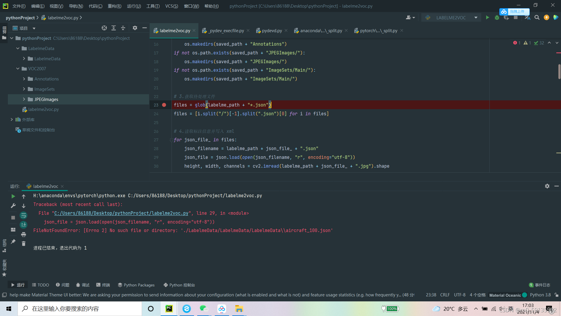
A small problem in labelme to VOC code
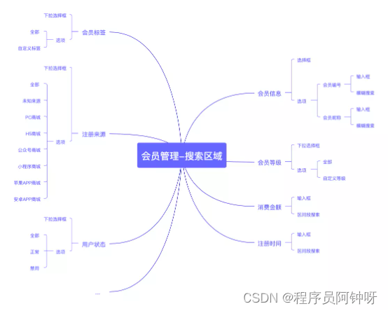
Multi merchant mall system function disassembly lecture 13 - platform side member management
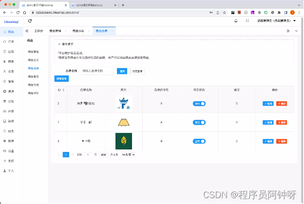
多商户商城系统功能拆解09讲-平台端商品品牌

Add se channel attention module to the network

多商户商城系统功能拆解05讲-平台端商家主营类目
随机推荐
Typora 安装包2021年11月最后一次免费版本的安装包下载V13.6.1
学习率余弦退火衰减之后的loss
Could not load library cudnn_cnn_infer64_8.dll. Error code 126Please make sure cudnn_cnn_infer64_8.
Multi merchant mall system function disassembly Lecture 14 - platform side member level
多商户商城系统功能拆解14讲-平台端会员等级
likeshop单商户商城系统搭建,代码开源无加密
Inventory of well-known source code mall systems at home and abroad
【深度学习】手写神经网络模型保存
Multi merchant mall system function disassembly lecture 08 - platform end commodity classification
多商户商城系统功能拆解03讲-平台端商家管理
Multi merchant mall system function disassembly lecture 13 - platform side member management
学习率优化策略
"Statistical learning methods (2nd Edition)" Li Hang Chapter 17 latent semantic analysis LSA LSI mind mapping notes and after-school exercise answers (detailed steps) Chapter 17
systemctl + journalctl
What do programmers often mean by API? What are the API types?
Likeshop100%开源无加密-B2B2C多商户商城系统
《统计学习方法(第2版)》李航 第16章 主成分分析 PCA 思维导图笔记 及 课后习题答案(步骤详细)PCA 矩阵奇异值 第十六章
Loss after cosine annealing decay of learning rate
如何解决训练集和测试集的分布差距过大问题
Chapter 5 neural network