将一维数据(序列)转化为二维数据(图像)的方法汇总GAFS, MTF, Recurrence plot,STFT

将一维序列数据转化为二维图像数据的方法汇总 详细 全面

• 一、背景
• 二、方法介绍
• • 格拉米角场 GAFs
  • • 原理
    • 实现步骤
    • 调用示例
  • 马尔可夫变迁场 MTF
  • • 原理
    • 实现步骤
    • 调用示例
  • 递归图 Recurrence Plot
  • • 原理
    • 调用示例
  • 短时傅里叶变换 STFT
  • 原理
  • 实现步骤
  • 调用示例
• References
• 总结

一、背景

虽然深度学习方法(1D CNN, RNN, LSTM 等)可以直接处理一维数据，但是当前的深度学习方法主要还是处理二维结构数据的，特别是在计算机视觉CV以及自然语言处理NLP领域，各种各样的方法层出不穷。因此，如果能够将一维序列数据转化为二维(图像)数据, 则可以直接结合CV以及NLP领域的方法，是不是很有趣！

二、方法介绍

格拉米角场 GAFs

原理

将缩放后的1D序列数据从直角坐标系统转换到极坐标系统，然后通过考虑不同点之间的角度和/差以识别不同时间点的时间相关性。取决于是做角度和还是角度差，有两种实现方法：GASF(对应做角度和), GADF(对应做角度差)。

实现步骤

Step 1：缩放，将数据范围缩放到[-1,1]或者[0, 1], 公式如下：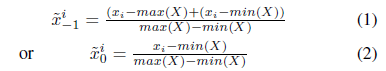

Step 2: 将缩放后的序列数据转换到极坐标系统，即将数值看作夹角余弦值，时间戳看作半径，公式如下：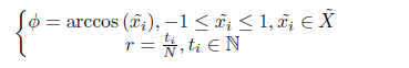

注： 若数据缩放范围为[-1, 1],则转换后的角度范围为[0, π pi π]；若缩放范围为[0, 1]，则转换后的角度范围为[0, π pi π/2]。
Step 3:

可以看到，最终GASF和GADF的计算转化到直角坐标系下变成了“类似”内积的操作。

效率问题：对于长度为n的序列数据，转换后的GAFs尺寸为[n, n]的矩阵，可以采用PAA(分段聚合近似)先将序列长度减小，然后在转换。 所谓的PAA就是：将序列分段，然后通过平均将每个段内的子序列压缩为一个数值, 简单吧！

调用示例

Python工具包pytl中已经提供了API，另外，笔者自行实现代码, 想要查看实现细节以及获取更多测试用例，可从我的 链接获取。

'''
EnvironmentPython 3.6,  pyts: 0.11.0, Pandas: 1.0.3
'''
from mpl_toolkits.axes_grid1 import make_axes_locatable
from pyts.datasets import load_gunpoint
from pyts.image import GramianAngularField
# call API
X, _, _, _ = load_gunpoint(return_X_y=True)
gasf = GramianAngularField(method='summation')
X_gasf = gasf.transform(X)
gadf = GramianAngularField(method='difference')
X_gadf = gadf.transform(X)

plt.figure()
plt.suptitle('gunpoint_index_' + str(0))
ax1 = plt.subplot(121)
ax1.plot(np.arange(len(rescale(X[k][:]))), rescale(X[k][:]))
plt.title('rescaled time series')
ax2 = plt.subplot(122, polar=True)
r = np.array(range(1, len(X[k]) + 1)) / 150
theta = np.arccos(np.array(rescale(X[k][:]))) * 2 * np.pi  # radian -> Angle

ax2.plot(theta, r, color='r', linewidth=3)
plt.title('polar system')
plt.show()

plt.figure()
plt.suptitle('gunpoint_index_' + str(0))
ax1 = plt.subplot(121)
plt.imshow(X_gasf[k])
plt.title('GASF')
divider = make_axes_locatable(ax1)
cax = divider.append_axes("right", size="5%", pad=0.2) # Create an axes at the given *position*=right with the same height (or width) of the main axes
plt.colorbar(cax=cax)

ax2 = plt.subplot(122)
plt.imshow(X_gadf[k])
plt.title('GASF')
divider = make_axes_locatable(ax2)
cax = divider.append_axes("right", size="5%",
                          pad=0.2)  # Create an axes at the given *position*=right with the same height (or width) of the main axes
plt.colorbar(cax=cax)
plt.show()

结果如下图所示：
缩放后的序列数据以及在极坐标系统的表示：

转换后的GASF和GADF:

---

马尔可夫变迁场 MTF

原理

基于1阶马尔可夫链，由于马尔科夫转移矩阵对序列的时间依赖并不敏感，因此作者考虑了时间位置关系提出了所谓的MTF。

实现步骤

Step 1: 首先将序列数据(长度为n)按照其取值范围划分为Q个bins (类似于分位数), 每个数据点 i 属于一个唯一的qi ( ∈ in ∈ {1,2, …, Q}).
Step 2: 构建马尔科夫转移矩阵W，矩阵尺寸为：[Q, Q]， 其中W[i，j]由qi中的数据被qj中的数据紧邻的频率决定，其计算公式如下：
w i , j = ∑ x ∈ q i , y ∈ q j , x + 1 = y 1 / ∑ j = 1 Q w i , j w_{i,j}=sum_{ orall x in q_{i}, y in q_{j},x+1=y}1/sum_{j=1}^{Q}w_{i,j} wi,j=∑x∈qi,y∈qj,x+1=y1/∑j=1Qwi,j
Step 3:构建马尔科夫变迁场M, 矩阵尺寸为：[n, n], M[i,j]的值为W[qi, qj]

效率问题：原因与GAFs类似，为了提高效率，设法减小M的尺寸，思路与PAA类似，将M网格化，然后每个网格中的子图用其平均值替代。

调用示例

Python工具包pytl中已经提供了API，API接口参考：https://pyts.readthedocs.io/en/latest/generated/pyts.image.MarkovTransitionField.html。另外，笔者自行实现代码, 想要查看实现细节以及获取更多测试用例，可从我的 github 链接获取。

'''
EnvironmentPython 3.6,  pyts: 0.11.0, Pandas: 1.0.3
'''
from mpl_toolkits.axes_grid1 import make_axes_locatable
from pyts.datasets import load_gunpoint
from pyts.image import MarkovTransitionField
## call API
X, _, _, _ = load_gunpoint(return_X_y=True)
mtf = MarkovTransitionField()
fullimage = mtf.transform(X)

# downscale MTF of the time series (without paa) through mean operation
batch = int(len(X[0]) / s)
patch = []
for p in range(s):
    for q in range(s):
        patch.append(np.mean(fullimage[0][p * batch:(p + 1) * batch, q * batch:(q + 1) * batch]))
# reshape
patchimage = np.array(patch).reshape(s, s)

plt.figure()
plt.suptitle('gunpoint_index_' + str(k))
ax1 = plt.subplot(121)
plt.imshow(fullimage[k])
plt.title('full image')
divider = make_axes_locatable(ax1)
cax = divider.append_axes("right", size="5%", pad=0.2)
plt.colorbar(cax=cax)

ax2 = plt.subplot(122)
plt.imshow(patchimage)
plt.title('MTF with patch average')
divider = make_axes_locatable(ax2)
cax = divider.append_axes("right", size="5%", pad=0.2)
plt.colorbar(cax=cax)
plt.show()

结果如图所示：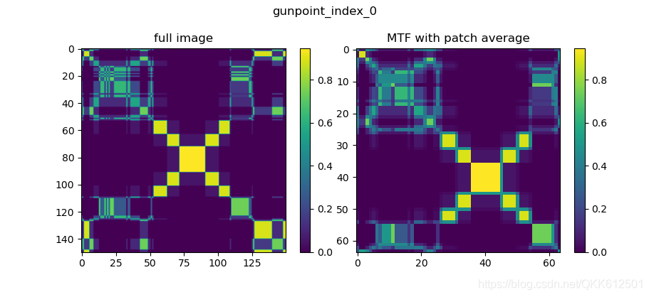

---

递归图 Recurrence Plot

递归图(recurrence plot，RP)是分析时间序列周期性、混沌性以及非平稳性的一个重要方法，用它可以揭示时间序列的内部结构，给出有关相似性、信息量和预测性的先验知识，递归图特别适合短时间序列数据，可以检验时间序列的平稳性、内在相似性。

原理

递归图是表示从原始时间序列提取的轨迹之间的距离的图像
给定时间序列数据: ( x 1 , … , x n ) (x_1, ldots, x_n) (x1,…,xn),提取到的轨迹为：
x i = ( x i , x i + τ , … , x i + ( m 1 ) τ ) , i ∈ { 1 , … , n ( m 1 ) τ } ec{x}_i = (x_i, x_{i + au}, ldots, x_{i + (m - 1) au}), quad orall i in {1, ldots, n - (m - 1) au } x i=(xi,xi+τ,…,xi+(m1)τ),i∈{1,…,n(m1)τ}
其中： m m m是轨迹的维数， τ au τ是时延。 递归图R是轨迹之间的成对距离，计算如下：
R i , j = Θ ( ε ∥ x i x j ∥ ) , i , j ∈ { 1 , … , n ( m 1 ) τ } R_{i, j} = Theta(arepsilon - | ec{x}_i - ec{x}_j |), quad orall i,j in {1, ldots, n - (m - 1) au } Ri,j=Θ(ε∥x ix j∥),i,j∈{1,…,n(m1)τ}
其中， Θ Theta Θ为Heaviside函数，而 ε arepsilon ε 是阈值。

调用示例

'''
EnvironmentPython 3.6,  pyts: 0.11.0, Pandas: 1.0.3
'''
from mpl_toolkits.axes_grid1 import make_axes_locatable
from pyts.datasets import load_gunpoint
from pyts.image import RecurrencePlot

X, _, _, _ = load_gunpoint(return_X_y=True)
rp = RecurrencePlot(dimension=3, time_delay=3)
X_new = rp.transform(X)
rp2 = RecurrencePlot(dimension=3, time_delay=10)
X_new2 = rp2.transform(X)
plt.figure()
plt.suptitle('gunpoint_index_0')
ax1 = plt.subplot(121)
plt.imshow(X_new[0])
plt.title('Recurrence plot, dimension=3, time_delay=3')
divider = make_axes_locatable(ax1)
cax = divider.append_axes("right", size="5%", pad=0.2)
plt.colorbar(cax=cax)

ax1 = plt.subplot(122)
plt.imshow(X_new2[0])
plt.title('Recurrence plot, dimension=3, time_delay=10')
divider = make_axes_locatable(ax1)
cax = divider.append_axes("right", size="5%", pad=0.2)
plt.colorbar(cax=cax)
plt.show()

结果如图：

---

短时傅里叶变换 STFT

STFT可看作一种量化非平稳信号的频率和相位含量随时间变化的方式。.

原理

通过添加窗函数（窗函数的长度是固定的），首先对时域信号加窗，通过滑动窗口的方式将原始时域信号分割为多个片段，然后对每一个片段进行FFT变换，从而得到信号的时频谱（保留了时域信息）。

实现步骤

假设序列的长度为 T T T, τ au τ为窗口窗口长度, s s s为滑动步长，W表示窗函数, 则STFT可以计算为：

S T F T ( τ , s ) ( X ) [ m , k ] = ∑ t = 1 T X [ t ] W ( t s m ) e x p { j 2 π k / τ ( t s m ) } STFT^{( au,s)}(X)_{[m,k]}=sum_{t=1}^{T}X_{[t]} cdot W(t-sm)cdot exp{-j2pi k / au cdot (t-sm)} STFT(τ,s)(X)[m,k]=∑t=1TX[t]W(tsm)exp{j2πk/τ(tsm)}

变换后的STFT尺寸为：[M, K], M代表时间维度，K代表频率幅值(复数形式),为方便起见，假设 s = τ s= au s=τ, 即窗口之间没有重叠，则
M = T / τ M=T/ au M=T/τ，
K = τ K =lfloor au floor K=τ/2 + 1

注：相比于DFT, STFT在某种程度上帮助我们恢复时间分辨率，然而在可达到的时间分辨率和频率之间会发生权衡，这就是所谓的不确定性原理。具体来说，窗口的宽度（ τ au τ）越大，频域分辨率就越高，相应地，时域分辨率越低；窗口的宽度（ τ au τ）越小，频域分辨率就越低，相应地，时域分辨率越高。

调用示例

python包 scipy提供STFT的API,具体官方文档介绍见：https://docs.scipy.org/doc/scipy/reference/generated/scipy.signal.stft.html

scipy.signal.stft(x，fs = 1.0，window =‘hann’，nperseg = 256，noverlap = None，nfft = None，detrend = False，return_oneside = True，boundary
=‘zeros’，padded = True，axis = -1 ）

参数解释：
x： 时域信号；
fs： 信号的采样频率；
window： 窗函数；
nperseg： 窗函数长度；
noverlap： 相邻窗口的重叠长度，默认为50%；
nfft： FFT的长度，默认为nperseg。如大于nperseg会自动进行零填充；
return_oneside ： True返回复数实部，None返回复数。
示例代码：

"""
@author: masterqkk, [email protected]
Environment:
    python: 3.6
    Pandas: 1.0.3
    matplotlib: 3.2.1
"""
import pickle
import numpy as np
import matplotlib.pyplot as plt
import scipy.signal as scisig
from mpl_toolkits.axes_grid1 import make_axes_locatable
from pyts.datasets import load_gunpoint

if __name__ == '__main__':
    X, _, _, _ = load_gunpoint(return_X_y=True)

    fs = 10e3  # sampling frequency
    N = 1e5  # 10 s 1signal
    amp = 2 * np.sqrt(2)
    time = np.arange(N) / float(fs)
    mod = 500 * np.cos(2 * np.pi * 0.25 * time)
    carrier = amp * np.sin(2 * np.pi * 3e3 * time + mod)
    noise_power = 0.01 * fs / 2
    noise = np.random.normal(loc=0.0, scale=np.sqrt(noise_power), size=time.shape)
    noise *= np.exp(-time / 5)
    x = carrier + noise  # signal with noise

    per_seg_length = 1000 # window length
    f, t, Zxx = scisig.stft(x, fs, nperseg=per_seg_length, noverlap=0, nfft=per_seg_length, padded=False)
    print('Zxx.shaope: {}'.format(Zxx.shape))  

    plt.figure()
    plt.suptitle('gunpoint_index_0')
    ax1 = plt.subplot(211)
    ax1.plot(x)
    plt.title('signal with noise')

    ax2 = plt.subplot(212)
    ax2.pcolormesh(t, f, np.abs(Zxx), vmin=0, vmax=amp)
    plt.title('STFT Magnitude')
    ax2.set_ylabel('Frequency [Hz]')
    ax2.set_xlabel('Time [sec]')
    plt.show()

运行结果：
得到STFT结果尺寸为：
Zxx.shaope: (501, 101)， 频率成分的数量为 1000 lfloor 1000 floor 1000/2 + 1 = 501， 窗口片段的长度为1e5/1000 + 1=101 (此处应该是进行了pad)

References

1.Imaging Time-Series to Improve Classification and Imputation
2.Encoding Time Series as Images for Visual Inspection and Classification Using Tiled Convolutional Neural Networks
3.J.-P Eckmann, S. Oliffson Kamphorst and D Ruelle, “Recurrence Plots of Dynamical Systems”. Europhysics Letters (1987)
4.Stoica, Petre, and Randolph Moses,Spectral Analysis of Signals, Prentice Hall, 2005
5.https://laszukdawid.com/tag/recurrence-plot/

总结

最后附上时间序列数据集下载链接：http://www.cs.ucr.edu/~eamonn/time_series_data/, 几乎包含了所有当前该领域的数据集。
希望能帮助到大家， 未完待续。欢迎交流：[email protected]