Learning strategies of 2D target detection overview (final chapter)

One 、 Training phase

      In this part , We review several learning strategies for training target detectors . Specifically, it includes data optimization 、 Unbalanced sampling 、 Positioning refinement and other learning strategies .

1. Data to enhance

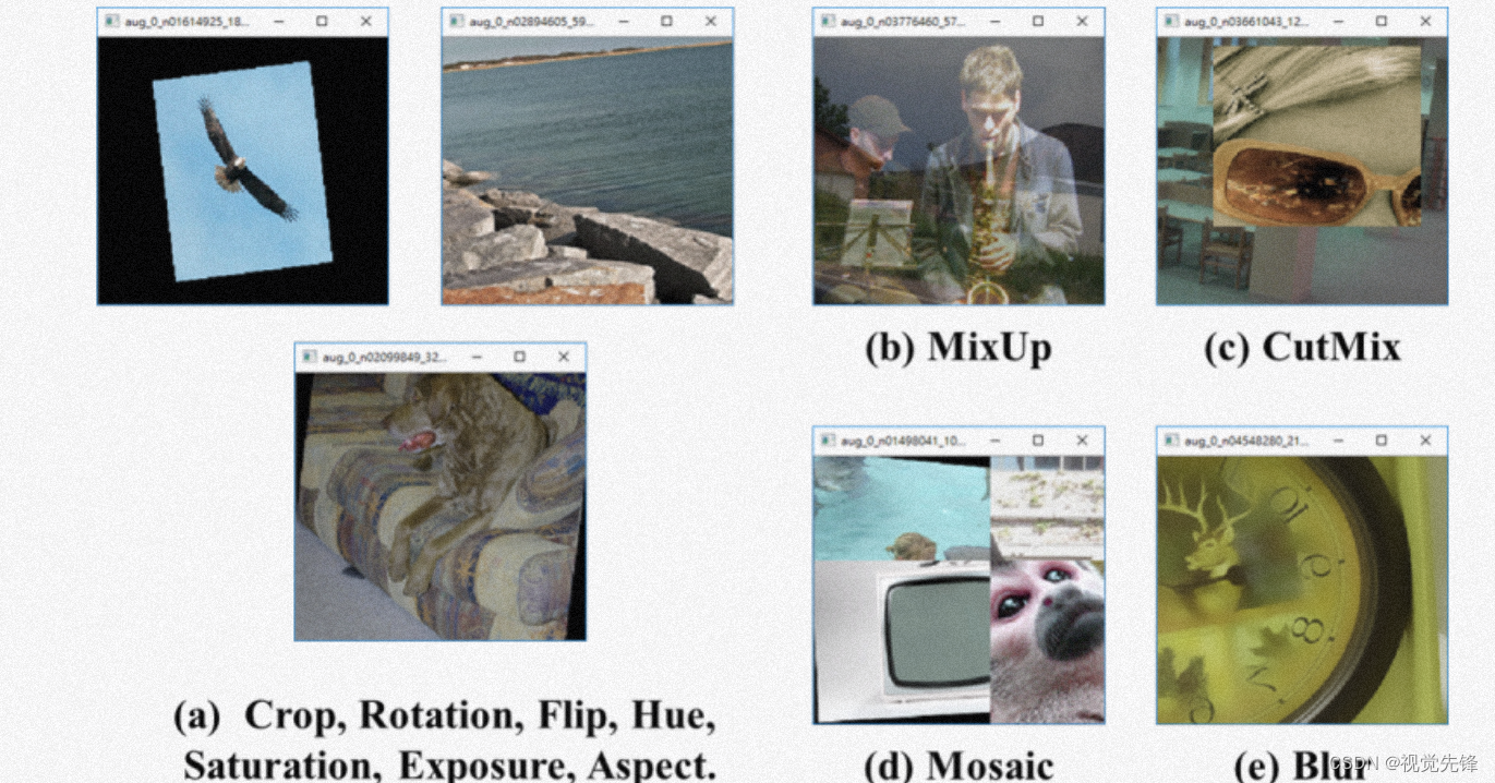
        Data enhancement is important for almost all deep learning methods , Because they usually need a lot of data , More training data will produce better results . In target detection , In order to increase training data and generate training pictures with various visual characteristics ,Faster R-CNN The method of horizontal turnover is used . A more intensive data enhancement strategy is used in the single-stage detector , Including rotation 、 Random cutting 、 Expansion and color jitter . These enhancement strategies have significantly improved the detection accuracy .（albumentations The package contains a lot of data, and the enhancement methods can be used directly ）

 

 

• Geometric enhancement ： Including translation 、 rotate 、 Cutting and other geometric changes to the image , It can enhance the generalization ability of the model .
• Color enhancement ： Mainly the brightness transformation , If you use HSV enhance .
• blurred ： Such as Gaussian filtering 、 Box filtering 、 Median filtering, etc . It can enhance the generalization ability of the model to blurred images .
• mixup： The above general data enhancement method is to transform the same class , and mixup Data enhancement is achieved by modeling different categories . Different classes with different weights , The loss function obtained is also added with different weights , Finally, the parameters are calculated by back propagation .
• Random erase ： The main purpose of this paper is to simulate occlusion , So as to improve the robustness of the model to occlusion . Randomly select an area , And then cover it with random values , Simulate an occluded scene .
• CutOut： Its purpose is the same as random erasure , Also simulate occlusion , By randomly selecting a square area of fixed size , Then use full 0 Just fill in . To avoid filling 0 The effect of value on training , Data should be normalized centrally .
• CutMix： Is to put a part of the area cut fall , But don't fill 0 value , Instead, it randomly fills the region pixel values of other data in the training set , The classification results are distributed in a certain proportion .
• Mosaic：cutmix Use two pictures , and mosaic Use four pictures , The advantage is that it enriches the background of object detection , And in BN When calculating, I will calculate at once 4 Picture data , bring mini-batch It doesn't need to be too big , stay GPU Get more efficient results on .

 2. Validation set partition

• Direct division ： The way of random division may make the training data and test data of the model very different , The generalization ability of the trained model is not strong .
• LOOCV（Leave－one－out Cross Validation）： This is a K A special case of folded cross validation , namely K＝N. Use only one data at a time as a test , Others are training sets , repeat N Time （N Is the number of samples in the dataset ）.
• KFold： Each test set will no longer contain only one data , It's more than one. , The specific number will be regarded as K Depends on your choice . for example , if K＝5, be 5 The process of cross validation is ：（1） Divide all data sets into 5 Share （2） Take one of them every time without repetition to make a test set , The other four are used as training sets and training models , Then calculate the error rate of the model on each test set （3） take 5 The error rate of times is averaged to the final error rate .

3. Unbalanced sampling

        In target detection , The imbalance between positive and negative samples is a key problem . in other words , Most of the regions of interest estimated as proposals are actually just background images . Few of them are positive samples . This leads to an imbalance problem when training the detector . say concretely , There are two problems to be solved ： Category imbalance （class imbalance） And difficulty imbalance （difficulty imbalance）. The so-called category imbalance , It means that most of the candidate proposals belong to the background , Only a few proposals contain goals . This leads to background information dominating the gradient during training . The difficulty imbalance is closely related to the first problem , Due to category imbalance , This makes background proposals easier to classify , And goals become more difficult to classify . For the problem of difficulty imbalance , There are many strategies to solve it . Some two-stage detectors , Such as R－CNN and Fast R－CNN, Most negative samples will be rejected first , And keep 2000 Proposals for further classification .

        stay Fast R－CNN in , The author starts with 2000 Negative samples are randomly selected from the proposals , Every batch The proportion of positive and negative samples is 1：3, To further eliminate the adverse effects of category imbalance . The disadvantage of this method is that it cannot make full use of the information of negative sample proposals , Some negative sample proposals may contain rich contextual information , And some hard negative proposals （hard negative proposals） It can help improve the detection accuracy . Therefore, some people have proposed a hard negative sampling strategy , This strategy fixes the ratio of foreground to background , But the most difficult negative proposal was sampled to update the model . say concretely , Choose the negative proposal with higher classification loss to train the model .

        In order to solve the problem of difficulty imbalance , Most sampling strategies have carefully designed loss functions . For target detection , The classifier is in C＋1 Study on categories （C Target categories and 1 Background categories ）. Suppose the real category label of this area is u,p Is the classifier in C＋1 Discrete probability distributions of outputs on classes （p＝{p0,...,pC}）. The loss function is as follows ：

Someone also proposed a new loss function called focusing loss , It can suppress the signal of simple samples in negative samples . It does not discard all simple samples , Instead, assign importance weights to each sample , Its loss function is as follows ：

among α and γ It is a parameter that controls the importance weight . This makes the training process more focused on difficult proposals .

        For more details about loss functions, please refer to the following links ：

Distance-IoU Loss: Faster and Better Learning for Bounding Box Regression

Generalized Intersection over Union: A Metric and A Loss for Bounding BoxRegression

Bounding Box Regression with KL Loss

Towards Accurate One-Stage Object Detection with AP-Loss

DR Loss: Improving Object Detection by Distributional Ranking

4. Positioning refinement （localization refinement）

        The target detector must provide close location prediction for each target （bbox or mask）. Many works have been improved . Precise positioning is challenging , Because the prediction results usually focus on the most recognizable part of the object , Not necessarily the area containing objects . In some scenes , High quality algorithms are needed to make high-quality predictions （ high IoU threshold ）, As shown in the figure below , It shows how the detector works at high IoU Failure under threshold conditions .

In this section, we will review some methods to refine the positioning results . stay R－CNN in , We learned L2 Auxiliary bounding box regressor to optimize positioning . stay Fast R-CNN in , Learn smooth through an end-to-end approach L1 Regressor , As shown below ：

among tc Represents the offset predicted for each target category ,v Represents the truth bounding box .x,y,z,w Represent the central coordinates and width of the bounding box respectively 、 high .

5. Cascade learning ：

        Cascade learning is a learning strategy from rough to fine , It collects information from the output of a given classifier , Build stronger classifiers in a cascading way . In recent years , Cascade learning is also applied to detection tasks based on deep learning , Especially detect small objects in large scenes . In addition to accelerating the algorithm , Cascading learning can also integrate contextual information , Improve positioning accuracy .

      There are other learning strategies that provide us with new directions , But it has not been widely explored at present . Mainly divided into the following categories ：

• Against learning ： Confrontational learning has made great progress in generating models . The most famous work of applied confrontation learning is generating confrontation Networks （GAN）, The generator and discriminator are competitive . The generator takes the noise vector as input , Generate false images to touch your data distribution , And use these false images to confuse the discriminator , The discriminator needs to recognize the real image from the data with false image .GAN Many variants of have shown good performance in many fields . Some people suggest using GAN Small target detection . The generator learns the high-resolution feature representation of small targets . say concretely , The generator converts low resolution small areas into high-resolution features , And compete with discriminators that recognize real high-resolution . Finally, the generator learns to generate high-quality features of small objects .
• Train from the beginning ： Modern target detectors mostly rely on ImageNet Pre trained classification model , However , The deviation of loss function and data distribution between classification and detection may adversely affect performance . Fine tuning the detection task can alleviate this problem , But the deviation cannot be completely eliminated . Besides , Moving the classification model to new areas for detection may bring more challenges . For these reasons , You need to train the detector from scratch , Instead of relying on the pre training model . The difficulty of training detectors from scratch is that the training data of target detection is usually insufficient , And may lead to over fitting . Unlike image classification , Object detection requires bounding box level annotations , therefore , Annotating large-scale test data sets takes a lot of time .
• Refine knowledge ： Through the teacher-student training program, the knowledge in the model set is extracted into a single model . This learning strategy is first used in image classification . In terms of target detection , Someone proposed a faster method based on R－CNN The detector , The detector is optimized through the training program of teachers and students . Use R－CNN The model acts as a classroom network to guide the training process . Compared with the traditional single model optimization strategy , Their framework has improved the detection accuracy . 

  Two 、 Testing phase

        The target detection algorithm produces a dense set of predictions , So due to a lot of repetition , These predictions cannot be directly used for evaluation . Besides , Some other learning strategies are needed to further improve the detection accuracy . These strategies improve the prediction quality or speed up the reasoning .

1. Remove redundancy

        Non maximum suppression （NMS） It is an integral part of target detection , False positive sample prediction for de duplication . As shown in the figure below ：

The target detection algorithm generates a dense set of predictions , It contains multiple repeated predictions . For single-stage Detection Algorithm , They generate a dense set of candidate proposals , Such as SSD or DSSD. Proposals around the same goal may have similar confidence , This leads to false positives . For the two-stage detection algorithm that generates sparse proposals , The bounding box regressor will bring the proposal closer to the same goal , This leads to the same problem . Repeated predictions are considered false positives , And will be punished in the prediction process , Therefore need NMS To eliminate these duplicate predictions . say concretely , For each category , Sort the prediction box according to the confidence score , And select the box with the highest score . Write it down as M. And then calculate M With other boxes IoU value , If IoU The value is greater than the preset threshold , Then these bounding boxes will be removed , The corresponding confidence score will also be reset to 0. Repeat this process for all prediction results .

  However , If the target happens to exist in M Of Ω within ,NMS It will cause the prediction to be lost , This situation is very common in cluster object detection . One solution to this problem is Soft－NMS. It will not directly eliminate B, It's going to be B The confidence decay of is its relationship with M Overlapping continuous functions F（F It can be a linear function or a Gaussian function ）, as follows ：

2. Model acceleration

（1） Calculation of shared characteristic graph ： In different stages of the target detector , Feature extraction is usually dominant . For sliding window based detectors , Computational redundancy starts with location and scale . The former is caused by the overlap between adjacent windows , The latter is caused by the feature correlation between adjacent scales .

• Redundancy and acceleration of spatial computing ： The most common method to reduce the redundancy of spatial computation is the shared computation of characteristic graphs , That is, before sliding the window , Calculate the feature map only once for the whole image . for example , In order to speed up HOG Speed of pedestrian detector , Researchers usually accumulate the entire input image HOG chart , As shown in the figure below ：

However , The disadvantages of this method are also obvious , That is, the resolution of the feature map will be affected cell Size limit . If a small object lies between two cell Between , It may be ignored .

        The idea of characteristic graph sharing computation is also widely used in convolution detectors . Most are based on CNN The detector , Such as SPPNET、Fast R-CNN And others have applied similar ideas , It achieves tens or even hundreds of times acceleration .

• Redundancy and acceleration of proportional calculation ： In order to reduce the redundancy of proportional calculation , The most successful method is to scale features directly instead of images . However , Due to the fuzzy effect , Such a method cannot be directly applied to things like HOG Such features . For this question , Researchers found through extensive statistics and analysis HOG The strong correlation between the adjacent scale of and the characteristics of the integral channel . This correlation can speed up the calculation of feature pyramid by approximating the feature map of adjacent scales . Besides , structure “ Detector pyramid ” It is another method to avoid proportional redundancy calculation , That is, simply slide multiple detectors on a feature map to detect objects of different scales , Instead of rescaling images or features .

（2） Network pruning and quantification ： “ Network pruning ” perhaps “ Network quantification ” It's acceleration CNN Two common techniques of model , The former refers to pruning the network structure or weight to reduce its size , The latter refers to the length of code that reduces activation or weight .

• Network pruning ： The research of network pruning was first carried out with a method called “ Best brain injury ” Method to compress the parameters of multilayer perceptron network . In this method , The loss function of the network is approximated by taking the second derivative , In order to remove some unimportant weights . According to this idea , In recent years, the network pruning method adopts the process of iterative training and pruning , That is, after each training stage , Remove a small number of unimportant weights , Repeat these operations . Because traditional network pruning only removes unimportant weights , This may lead to sparse connection patterns in convolution filters , Therefore, it cannot be directly applied to compression CNN Model . A simple solution to this problem is to delete the entire filter , Instead of independent weights .
• Network quantification ： Recently, the work on network quantization mainly focuses on network binarization , Its purpose is to quantify its activation or weight into binary variables （0／1） To speed up the network , Thus, the floating-point operation is converted into and 、 or 、 Unequal logic operation . Network binarization can significantly speed up computation and reduce network storage , So it is easier to deploy on mobile devices . A possible implementation of the above idea is to use the least square method to approximate convolution through binary variables . A more accurate approximation can be obtained by using a linear combination of multiple binary convolutions .

（3） Lightweight network design ： The last group accelerates CNN The method of detector is to design lightweight network , Instead of using an existing detection engine . For a long time , Researchers have been exploring the correct configuration of the network , In order to obtain higher accuracy in limited time . In addition to some general design principles , Such as fewer channels and more layers , In recent years, some other methods have been proposed , We will introduce .

• Factorization convolution ： The method is to build lightweight CNN The easiest way , There are two decomposition methods . 

        The first method is to decompose the large convolution filter into a group of small convolution filters in its spatial dimension , Pictured 14（b） Shown . for example , Can be 7×7 The filter is decomposed into 3 individual 3×3 filter , They share the same receptive field , But the latter is more effective . Another example is to put k×k The filter is decomposed into k×1 and 1×k filter , This is very effective for very large filters , At present, it has been applied to the field of target detection .

        The second method is to divide a group of large convolutions into two groups in the channel dimension , Pictured 14（c） Shown . for example , We can use one c Characteristic diagram and d A filter simulates a convolution , It can be broken down into d' A filter 、 A nonlinear activation layer and another d A filter （d'<d）.

• Grouping convolution ： The purpose of grouping convolution is to divide the characteristic channels into different groups to reduce the number of parameters in the convolution layer , Then convolute independently on each group , Pictured 14（d） Shown . If we divide the characteristic channel into m Group , Without changing other configurations , The computational complexity of convolution will be reduced to the previous 1／m.
• Depth independent convolution ： Pictured 14（e） Shown , Deep separable convolution is to build lightweight CNN A popular method of . When the number of groups is set to the number of channels , It can be regarded as a special case of block convolution . Suppose we have a d Convolution layers of filters and c Characteristic diagram of the channel . The size of each filter is k×k. For depth separable convolution , Every k×k×c The filter of is first divided into c A slice , The size of each slice is k×k×1, Then convolution is performed separately in each same channel using each slice of the filter . Finally, use multiple 1×1 The filter performs dimensional conversion , In order to finally output the required d passageway .
• Bottleneck design ： Compared with the previous layers , The bottleneck layer of neural network contains fewer nodes . It can be used to learn effective data coding of dimension reduction input , This has been widely used in depth automatic encoder . In recent years , Bottleneck design is widely used in designing lightweight Networks . In these methods , A common method is to compress the input layer of the detector , So that the amount of calculation is reduced from the beginning of detection . Another method is to compress the output of the detection engine to make the feature map thinner , So that it is more effective in the subsequent detection stage .

（4） Numerical acceleration

• Accelerate with integral image ：

        Image integration is an important method in image processing . It helps to quickly calculate the sum on the image sub region . The essence of image integration is the separability of convolution integral and differential in signal processing ：

  among , If dg（x）／dx It's a sparse signal , Then the convolution can be accelerated by the right part of the equation .

        besides , Image integration can also be used to accelerate more general features in target detection , For example, color histogram 、 Gradient histogram, etc . A typical example is by calculating integral HOG Figure to accelerate HOG. integral HOG The image does not accumulate pixel values in a traditional integral image , Instead, accumulate gradient directions in the image . As shown in the figure below ：

Because you can cell The histogram in is regarded as the sum of gradient vectors in a specific region , So by using the integral image , With constant computing overhead , Calculate the histogram of rectangular area at any position and size .

• Frequency domain acceleration

        Convolution can be accelerated in many ways , Among them, Fourier transform is a very practical choice . The theoretical basis of frequency domain accelerated convolution is the convolution theorem in signal processing , That is, under appropriate conditions , The Fourier transform of convolution of two signals makes the dot product in Fourier space . as follows ：

among ,F It's Fourier transform ,F^－1 It's the inverse Fourier transform ,I and W They are input image and filter ,* For convolution operations , The right centered circle is a dot product operation . In the field of target detection , We can use the following figure to show this acceleration process .

 

• Vector quantization

        Vector quantization is a classical quantization method in signal processing , It aims to simulate the distribution of big data through a group of small raw vectors . It can be used for data compression and accelerating the inner product operation in target detection . for example , Use vector quantization , Can be HOG Histograms are grouped and quantized into a set of original histogram vectors . Then in the detection phase , The inner product between the feature vector and the detection weight is realized by looking up the table . Because there is no floating-point multiplication and division in this process , The detection speed of the detector is increased by an order of magnitude .

• Reduced rank estimation

        In deep networks , The full connection layer is essentially the multiplication of two matrices . When the parameter matrix W more , The computational burden of the detector will be heavy . Reduced rank estimation is a method of accelerating matrix multiplication , The aim is to W Perform low rank decomposition ：