当前位置:网站首页>[deep learning] teach you to write "handwritten digit recognition neural network" hand in hand, without using any framework, pure numpy
[deep learning] teach you to write "handwritten digit recognition neural network" hand in hand, without using any framework, pure numpy
2022-07-24 05:56:00 【Meow, meow, hammer, you cute】
List of articles
Preface
I have always been interested in machine learning , But because the major of university has nothing to do with machine learning , So there has been no time ( Procrastination ) Write a neural network completely without a framework . Fortunately, there is a major elective course this semester , Take this opportunity to publish your learning achievements .
The premise of learning this article is that you have a certain Python、 linear algebra 、 Advanced mathematics knowledge , And have a certain understanding of fully connected neural networks , Know that the fully connected nerve is actually a The nonlinear function of any function can be approximated by adjusting parameters ( That's how I understand it , Of course, I also believe that there are many functions that it cannot accurately describe ), Know the process of forward and backward propagation .
If you know something about neural networks , But I didn't think about it carefully I suggest you take a look first B standing 3Blue1Brown About Deep learning Deep Learning In the video , After learning this video, you can be right All connected neural networks Have a deeper understanding . Of course, you may still not be able to write a complete neural network , Because many people may not know much about the derivation of matrix in the process of back propagation , As a result, the calculation formula of the gradient of the back propagation process cannot be derived .
Handwritten numeral recognition neural network design
Suppose you have seen the video , Or have a better understanding of this , Then we can start designing .
Here for the convenience of explanation and making the first The procedure is clear !!!, Don't use MINIST The data set . Here is a data set provided by the tutorial I studied , This data set looks like this , The content of the file is the picture data of handwritten digits , Equivalent to binary image . Naming rules : The numbers in the picture _ Serial number --> label_seq.txt. Next, use the tag to call the value of the number written in the picture . The focus now is not on data sets , So here is the function of loading data and . Click here to download the dataset .
#  function img2vector Convert the image to a vector
from numpy import *
from os import listdir

def img2vector(filename):
    returnVect = np.zeros((1, 1024))
    fr = open(filename)
    for i in range(32):
        lineStr = fr.readline()
        for j in range(32):
            returnVect[0, 32 * i + j] = int(lineStr[j])
    return returnVect

#  Read handwritten fonts txt data
def handwritingData(dataPath):
    hwLabels = []
    FileList = listdir(dataPath)  # 1  Get the contents of the table of contents
    m = len(FileList)
    np.Mat = np.zeros((m, 1024))
    for i in range(m):
        # 2  Parse the classification number from the file name
        fileNameStr = FileList[i]
        fileStr = fileNameStr.split('.')[0]  # take off .txt
        classNumStr = int(fileStr.split('_')[0])
        hwLabels.append(classNumStr)
        np.Mat[i, :] = img2vector(dataPath + '/%s' % fileNameStr)
    return np.Mat, hwLabels
Dataset use
Extract the dataset to the specified directory ,like this:
..
└ Work Folder
	└ Net.py
	  trainingDigits
      testDigits
#  Read training data
trainDataPath = "./trainingDigits"
trainMat, trainLabels = handwritingData(trainDataPath)

trainMat.shape -> (1934, 1024)
trainMat[i] The corresponding label is trainLabels[i]
Neural network design

Here is the model, which is like this , Pictured above , An input layer , Two hidden layers , Activate function selection Sigmod, The loss function selects the sum of squared errors function ( I call it that , I don't know what it's called ), This is shown below . It is suggested that the loss function should be the sum of squares of errors for the first time , Think this loss function is simple , It is convenient to seek guidance , Easy to learn , Later, we can make improvements on this basis .
Cost : cost , Here is what needs to be calculated Loss value .
S i g m o d ( x ) = 1 1 + e − x S i g m o d ′ ( x ) = S i g m o d ( x ) ( 1 − S i g m o d ( x ) ) Sigmod(x) = \frac{1}{1+e^{-x}} \\ Sigmod'(x) = Sigmod(x)(1 - Sigmod(x)) \\ Sigmod(x)=1+e−x1Sigmod′(x)=Sigmod(x)(1−Sigmod(x))
By mistake Bad flat Fang and Letter Count : C o s t ( y ^ , y ) = 1 2 ( y ^ − y ) 2 Function of sum of squares of errors : Cost( \hat{y} , y) = \frac{1}{2} ( \hat{y} - y)^2 By mistake Bad flat Fang and Letter Count :Cost(y^,y)=21(y^−y)2
If the mathematical ability is not strong enough, it is recommended not to use cross entropy loss function , Don't use Softmax Activation function these functions with troublesome derivation , It's not good for learning .
mathematical model
operator Number : A ( layer ) Symbol :A^{( layer )} operator Number :A( layer )
S = S i g m o d S = Sigmod S=Sigmod
dimension degree : ∣ x 1024 x 1 ∣ W 16 x 1024 ( 1 ) ∣ b 16 x 1 ( 1 ) ∣ W 16 x 16 ( 2 ) ∣ b 16 x 1 ( 2 ) ∣ W 10 x 16 ( 3 ) ∣ b 10 x 1 ( 3 ) ∣ y ^ 10 x 1 ∣ dimension : | \boldsymbol{x}_{1024x1} | \boldsymbol{W}_{16x1024}^{(1)} | \boldsymbol{b}_{16x1}^{(1)} | \boldsymbol{W}_{16x16}^{(2)} | \boldsymbol{b}_{16x1}^{(2)} | \boldsymbol{W}_{10x16}^{(3)} | \boldsymbol{b}_{10x1}^{(3)} | \boldsymbol{\hat{y}_{10x1}} | dimension degree :∣x1024x1∣W16x1024(1)∣b16x1(1)∣W16x16(2)∣b16x1(2)∣W10x16(3)∣b10x1(3)∣y^10x1∣
front towards Pass on seeding : Forward propagation : front towards Pass on seeding :
z ( l ) = W ( l ) a ( l − 1 ) + b ( l ) \mathbf{z}^{(l)}=\mathbf{W}^{(l)} \mathbf{a}^{(l-1)}+\mathbf{b}^{(l)} z(l)=W(l)a(l−1)+b(l)
a ( l ) = f ( z ( l ) ) \mathbf{a}^{(l)}=f\left(\mathbf{z}^{(l)}\right) a(l)=f(z(l))
y ^ = a ( L ) = f ( z ( L ) ) \hat{\mathbf{y}}=\mathbf{a}^{(L)}=f\left(\mathbf{z}^{(L)}\right) y^=a(L)=f(z(L))
L = L ( y , y ^ ) \mathcal{L}=\mathcal{L}(\mathbf{y}, \hat{\mathbf{y}}) L=L(y,y^)
x = a ( 0 ) also Just yes transport Enter into Of chart slice Count According to the \boldsymbol{x} = a^{(0)} That is, the input image data x=a(0) also Just yes transport Enter into Of chart slice Count According to the
z ( 1 ) = W ( 1 ) a ( 0 ) + b ( 1 ) \boldsymbol{z}^{(1)} = \boldsymbol{W}^{(1)}\boldsymbol{a}^{(0)}+\boldsymbol{b}^{(1)} z(1)=W(1)a(0)+b(1)
a ( 1 ) = S ( z ( 1 ) ) \boldsymbol{a}^{(1)} = S(\boldsymbol{z}^{(1)}) a(1)=S(z(1))
z ( 2 ) = W ( 2 ) a ( 1 ) + b ( 2 ) \boldsymbol{z}^{(2)} = \boldsymbol{W}^{(2)}\boldsymbol{a}^{(1)}+\boldsymbol{b}^{(2)} z(2)=W(2)a(1)+b(2)
a ( 2 ) = S ( z ( 2 ) ) \boldsymbol{a}^{(2)} = S(\boldsymbol{z}^{(2)}) a(2)=S(z(2))
z ( 3 ) = W ( 2 ) a ( 2 ) + b ( 3 ) \boldsymbol{z}^{(3)} = \boldsymbol{W}^{(2)}\boldsymbol{a}^{(2)}+\boldsymbol{b}^{(3)} z(3)=W(2)a(2)+b(3)
y ^ = S ( z ( 3 ) ) pre measuring junction fruit , most Big value Next mark Just yes pre measuring Of Count word junction fruit \boldsymbol{\hat{y}} = S(\boldsymbol{z}^{(3)}) Predicted results , The maximum subscript is the predicted numerical result y^=S(z(3)) pre measuring junction fruit , most Big value Next mark Just yes pre measuring Of Count word junction fruit
L o s s = C o s t ( y ^ , y ) Loss = Cost( \boldsymbol{\hat{y}} , \boldsymbol{y}) Loss=Cost(y^,y)
back towards Pass on seeding : ⊙ yes Yes Should be element plain phase ride Back propagation :\odot It's the multiplication of the corresponding elements back towards Pass on seeding :⊙ yes Yes Should be element plain phase ride
∂ L o s s ∂ y ^ \frac{\partial Loss}{\partial \boldsymbol{\hat{y}}} ∂y^∂Loss: Here is the derivation of the corresponding element
Output layer :
δ ( L ) = ∇ a ( L ) L ⊙ S ′ ( z ( L ) ) = ∂ L o s s ∂ y ^ ⊙ S ′ ( z ( L ) ) = ∂ L ∂ z ( L ) this in seek have to : ∂ L o s s ∂ y ^ ⊙ S ′ ( z ( 3 ) ) \boldsymbol{\delta}^{(L)}=\nabla_{\mathbf{a}^{(L)}} \mathcal{L} \odot S^{\prime}\left(\mathbf{z}^{(L)}\right) = \frac{\partial Loss}{\partial \boldsymbol{\hat{y}}} \odot S^{\prime}\left(\mathbf{z}^{(L)}\right) = \frac{\partial \mathcal{L} }{\partial \mathbf{z}^{(L)}}\\ Here we find : \frac{\partial Loss}{\partial \boldsymbol{\hat{y}}} \odot S^{\prime}\left(\mathbf{z}^{(3)}\right) δ(L)=∇a(L)L⊙S′(z(L))=∂y^∂Loss⊙S′(z(L))=∂z(L)∂L this in seek have to :∂y^∂Loss⊙S′(z(3))
Other layers apply formulas :
δ ( l ) = ( ( W ( l + 1 ) ) T δ ( l + 1 ) ) ⊙ S ′ ( z ( l ) ) ∂ L ∂ W ( l ) = δ ( l ) ( a ( l − 1 ) ) T ∂ L ∂ b ( l ) = δ ( l ) \boldsymbol{\delta}^{(l)}=\left(\left(\mathbf{W}^{(l+1)}\right)^{\mathrm{T}} \boldsymbol{\delta}^{(l+1)}\right) \odot S^{\prime}\left(\mathbf{z}^{(l)}\right) \\ \frac{\partial \mathcal{L}} {\partial\mathbf{W}^{(l)}}=\boldsymbol{\delta}^{(l)}\left(\mathbf{a}^{(l-1)}\right)^{\mathrm{T}} \\ \frac{\partial \mathcal{L}}{\partial \mathbf{b}^{(l)}}=\boldsymbol{\delta}^{(l)} δ(l)=((W(l+1))Tδ(l+1))⊙S′(z(l))∂W(l)∂L=δ(l)(a(l−1))T∂b(l)∂L=δ(l)
ginseng Count more new : Parameters are updated : ginseng Count more new :
W ( l ) = W ( l ) − α ∂ L ∂ W ( l ) b ( l ) = b ( l ) − α ∂ L ∂ b ( l ) \begin{aligned} \mathbf{W}^{(l)} &=\mathbf{W}^{(l)}-\alpha \frac{\partial \mathcal{L}}{\partial \mathbf{W}^{(l)}} \\ \mathbf{b}^{(l)} &=\mathbf{b}^{(l)}-\alpha \frac{\partial \mathcal{L}}{\partial \mathbf{b}^{(l)}} \end{aligned} W(l)b(l)=W(l)−α∂W(l)∂L=b(l)−α∂b(l)∂L
About matrix derivation
If you just want to be able to find out the gradient in the back propagation process by yourself , Then remember the above formula is enough , If you want to know more about the formula, you can refer to this article : Neural network derivation .
Scalar f f f The matrix X \boldsymbol{X} X The derivative of , Defined as ∂ f ∂ X = [ ∂ f ∂ X i j ] \frac{\partial f}{\partial X}=\left[\frac{\partial f}{\partial X_{i j}}\right] ∂X∂f=[∂Xij∂f].
Of course , You may not want to stop here , Maybe some students didn't contact matrix derivation and got stuck in the derivation of the back-propagation formula . If you want to know how to perform matrix derivation, you can refer to : Matrix derivation . Of course, there is a simple way , Is to write out the equation solved by each element of the matrix together with its subscript , like this : y i × 1 = ∑ j W i × j x j × 1 y_{i \times1} = \sum_{j} W_{i \times j} x_{j \times 1} yi×1=∑jWi×jxj×1. And then express the partial derivative , like this : ∂ y i × 1 ∂ W i × j = x j × 1 \frac{\partial y_{i \times1}}{\partial W_{i \times j} } = x_{j \times 1} ∂Wi×j∂yi×1=xj×1. It's equivalent to just W \mathbf{W} W Of the i i i That's ok W i × j \boldsymbol{W}_{i \times \boldsymbol{j}} Wi×j Made a contribution , and W \mathbf{W} W Of the i i i That's ok W i × j \boldsymbol{W}_{i \times \boldsymbol{j}} Wi×j(j It's equivalent to having a vector ) Only right y i × 1 y_{i \times1} yi×1 Contribute .
Make y i × 1 = W i × j x j × 1 + b i × 1 , y_{i \times1} = \boldsymbol{W}_{i \times \boldsymbol{j}}\boldsymbol{x}_{\boldsymbol{j} \times 1} + \boldsymbol{b}_{i \times 1}, yi×1=Wi×jxj×1+bi×1, hold W i × j Of Every time individual element plain W i × j \boldsymbol{W}_{i \times \boldsymbol{j}} Each element of W_{i \times j} Wi×j Of Every time individual element plain Wi×j As a variable , y i × 1 y_{i \times1} yi×1 Equivalent to a multivariate function , Elements W i × j W_{i \times j} Wi×j increase 1 Yes y i × 1 y_{i \times1} yi×1 The impact of this is Δ y i × 1 Δ W i × j \frac{\Delta y_{i \times1}}{\Delta W_{i \times j} } ΔWi×jΔyi×1, Take the limit as ∂ y i × 1 ∂ W i × j = x j × 1 \frac{\partial y_{i \times1}}{\partial W_{i \times j} } = x_{j \times 1} ∂Wi×j∂yi×1=xj×1, Because there is only number W \boldsymbol{W} W Of the i i i Column , Have an impact on , So the final gradient should be one line , The value of this line Transposition Namely x \boldsymbol{x} x. x \boldsymbol{x} x Take the derivative as a constant .
Say something reasonable. , Here's the picture : hypothesis i = 1 i = 1 i=1.
∂ y i × 1 ∂ W i × j = [ ∂ y 1 × 1 ∂ W 1 × 1 = x 1 × 1 ∂ y 1 × 1 ∂ W 1 × 2 = x 2 × 1 ⋯ ∂ y i × 1 ∂ W i × j = x j × 1 ] = [ x 1 × 1 x 2 × 1 ⋮ x j × 1 ] T = x T \frac{\partial {y}_{i \times1}}{\partial \boldsymbol{W}_{i \times \boldsymbol{j}} } = \left[ \begin{matrix} \frac{\partial y_{1 \times1}}{\partial W_{1 \times 1} } =x_{1 \times 1} & \frac{\partial y_{1 \times1}}{\partial W_{1 \times 2} } =x_{2 \times 1} & \cdots & \frac{\partial y_{i \times1}}{\partial W_{i \times j} } = x_{j \times 1} \\ \end{matrix} \right] \\ =\left[ \begin{matrix} x_{1 \times 1} \\ x_{2 \times 1} \\ \vdots \\ x_{j \times 1} \\ \end{matrix} \right]^T = \boldsymbol{x}^T ∂Wi×j∂yi×1=[∂W1×1∂y1×1=x1×1∂W1×2∂y1×1=x2×1⋯∂Wi×j∂yi×1=xj×1]=⎣⎢⎢⎢⎡x1×1x2×1⋮xj×1⎦⎥⎥⎥⎤T=xT
Of course , This proof is incomplete , I don't think the rest is necessary ( Don't bother ) Yes . Notice that this is the derivative of the variable to the matrix , although y \boldsymbol{y} y There are many , But they came separately . Again because L o s s Loss Loss Yes, yes y \boldsymbol{y} y The sum function , So according to the chain derivation rule :
y = W x L o s s = C ( y ) ∂ L o s s ∂ W = ∂ L o s s ∂ y ∂ y ∂ W \boldsymbol{y} = \boldsymbol{W} \boldsymbol{x} \\ Loss = C(\boldsymbol{y}) \\ \frac{\partial Loss }{\partial \boldsymbol{W} } = \frac{\partial Loss }{\partial \boldsymbol{y} } \frac{\partial \boldsymbol{y}}{\partial \boldsymbol{W} } y=WxLoss=C(y)∂W∂Loss=∂y∂Loss∂W∂y
∂ L o s s ∂ y \frac{\partial Loss }{\partial \boldsymbol{y} } ∂y∂Loss It's deriving item by item , Get vector δ \boldsymbol{\delta} δ Just put each ∂ y i × 1 ∂ W i × j \frac{\partial y_{i \times1}}{\partial W_{i \times j} } ∂Wi×j∂yi×1" Moved to " Corresponding rows .
∂ L o s s ∂ W = ∂ L o s s ∂ y x T \frac{\partial Loss }{\partial \boldsymbol{W} } = \frac{\partial Loss }{\partial \boldsymbol{y} } \boldsymbol{x}^T ∂W∂Loss=∂y∂LossxT
Complete parsing :
∂ L o s s ∂ W = ∂ L o s s ∂ y ∂ y ∂ W = [ ∂ L o s s ∂ y 1 × 1 ∂ y 1 × 1 ∂ W 1 × j ∂ L o s s ∂ y 2 × 1 ∂ y 2 × 1 ∂ W 2 × j ⋮ ∂ L o s s ∂ y i × 1 ∂ y i × 1 ∂ W i × j ] = [ ∂ L o s s ∂ y 1 × 1 ∂ y 1 × 1 ∂ W 1 × 1 = x 1 × 1 ∂ L o s s ∂ y 1 × 1 ∂ y 1 × 1 ∂ W 1 × 2 = x 2 × 1 ⋯ ∂ L o s s ∂ y 1 × 1 ∂ y 1 × 1 ∂ W 1 × j = x j × 1 ∂ L o s s ∂ y 2 × 1 ∂ y 2 × 1 ∂ W 2 × 1 = x 1 × 1 ∂ L o s s ∂ y 2 × 1 ∂ y 2 × 1 ∂ W 2 × 2 = x 2 × 1 ⋯ ∂ L o s s ∂ y 2 × 1 ∂ y 2 × 1 ∂ W 2 × j = x j × 1 ⋮ ⋮ ⋱ ⋮ ∂ L o s s ∂ y i × 1 ∂ y i × 1 ∂ W i × 1 = x 1 × 1 ∂ L o s s ∂ y i × 1 ∂ y i × 1 ∂ W i × 2 = x 2 × 1 ⋯ ∂ L o s s ∂ y i × 1 ∂ y i × 1 ∂ W i × j = x j × 1 ] = ∂ L o s s ∂ W = ∂ L o s s ∂ y ∂ y ∂ W = [ ∂ L o s s ∂ y 1 × 1 ∂ L o s s ∂ y 2 × 1 ⋮ ∂ L o s s ∂ y i × 1 ] [ x 1 × 1 x 2 × 1 ⋯ x j × 1 ] = ∂ L o s s ∂ y x T \frac{\partial Loss }{\partial \boldsymbol{W} } = \frac{\partial Loss }{\partial \boldsymbol{y} } \frac{\partial \boldsymbol{y}}{\partial \boldsymbol{W} } = \\ \left[ \begin{matrix} \frac{\partial Loss }{\partial {y_{1 \times 1}} } \frac{\partial {y}_{1 \times1}}{\partial \boldsymbol{W}_{1 \times \boldsymbol{j}} }\\ \frac{\partial Loss }{\partial {y_{2 \times 1}} } \frac{\partial {y}_{2 \times1}}{\partial \boldsymbol{W}_{2 \times \boldsymbol{j}} } \\ \vdots \\ \frac{\partial Loss }{\partial {y_{i \times 1}} } \frac{\partial {y}_{i \times1}}{\partial \boldsymbol{W}_{i \times \boldsymbol{j}} } \\ \end{matrix} \right] = \left[ \begin{matrix} \frac{\partial Loss }{\partial {y_{1 \times 1}} } \frac{\partial {y}_{1 \times1}}{\partial {W}_{1 \times {1}} } = x_{1 \times 1} & \frac{\partial Loss }{\partial {y_{1 \times 1}} } \frac{\partial {y}_{1 \times1}}{\partial {W}_{1 \times {2}} } = x_{2 \times 1} & \cdots & \frac{\partial Loss }{\partial {y_{1 \times 1}} } \frac{\partial {y}_{1 \times1}}{\partial {W}_{1 \times {j}} } = x_{j \times 1} \\ \frac{\partial Loss }{\partial {y_{2 \times 1}} } \frac{\partial {y}_{2 \times1}}{\partial {W}_{2 \times {1}} } = x_{1 \times 1} & \frac{\partial Loss }{\partial {y_{2 \times 1}} } \frac{\partial {y}_{2 \times1}}{\partial {W}_{2 \times {2}} } = x_{2 \times 1} & \cdots & \frac{\partial Loss }{\partial {y_{2 \times 1}} } \frac{\partial {y}_{2 \times1}}{\partial {W}_{2 \times {j}} } = x_{j \times 1} \\ \vdots & \vdots & \ddots & \vdots \\ \frac{\partial Loss }{\partial {y_{i \times 1}} } \frac{\partial {y}_{i \times1}}{\partial {W}_{i \times {1}} } = x_{1 \times 1} & \frac{\partial Loss }{\partial {y_{i \times 1}} } \frac{\partial {y}_{i \times1}}{\partial {W}_{i \times {2}} } = x_{2 \times 1} & \cdots & \frac{\partial Loss }{\partial {y_{i \times 1}} } \frac{\partial {y}_{i \times1}}{\partial {W}_{i \times {j}} } = x_{j \times 1} \\ \end{matrix} \right] \\ =\frac{\partial Loss }{\partial \boldsymbol{W} } = \frac{\partial Loss }{\partial \boldsymbol{y} } \frac{\partial \boldsymbol{y}}{\partial \boldsymbol{W} } = \\ \left[ \begin{matrix} \frac{\partial Loss }{\partial {y_{1 \times 1}} } \\ \frac{\partial Loss }{\partial {y_{2 \times 1}} } \\ \vdots \\ \frac{\partial Loss }{\partial {y_{i \times 1}} } \\ \end{matrix} \right] \left[ \begin{matrix} x_{1 \times 1} &x_{2 \times 1} & \cdots &x_{j \times 1} \end{matrix} \right] = \frac{\partial Loss }{\partial \boldsymbol{y} } \boldsymbol{x}^T ∂W∂Loss=∂y∂Loss∂W∂y=⎣⎢⎢⎢⎢⎡∂y1×1∂Loss∂W1×j∂y1×1∂y2×1∂Loss∂W2×j∂y2×1⋮∂yi×1∂Loss∂Wi×j∂yi×1⎦⎥⎥⎥⎥⎤=⎣⎢⎢⎢⎢⎡∂y1×1∂Loss∂W1×1∂y1×1=x1×1∂y2×1∂Loss∂W2×1∂y2×1=x1×1⋮∂yi×1∂Loss∂Wi×1∂yi×1=x1×1∂y1×1∂Loss∂W1×2∂y1×1=x2×1∂y2×1∂Loss∂W2×2∂y2×1=x2×1⋮∂yi×1∂Loss∂Wi×2∂yi×1=x2×1⋯⋯⋱⋯∂y1×1∂Loss∂W1×j∂y1×1=xj×1∂y2×1∂Loss∂W2×j∂y2×1=xj×1⋮∂yi×1∂Loss∂Wi×j∂yi×1=xj×1⎦⎥⎥⎥⎥⎤=∂W∂Loss=∂y∂Loss∂W∂y=⎣⎢⎢⎢⎢⎡∂y1×1∂Loss∂y2×1∂Loss⋮∂yi×1∂Loss⎦⎥⎥⎥⎥⎤[x1×1x2×1⋯xj×1]=∂y∂LossxT
I can't prove it mathematically , however , From the above derivation, it must be right . Of course, I recommend you to have a look Matrix derivation . Secondly, the above is the derivation of scalar to matrix or vector .
So you can probably see what the derivative looks like . I forgot how to deduce , But I have a better idea , From gradient ∇ \nabla ∇ Starting with .
Program realization
as follows , The initialization selection here can be all 1 Or all 0, But that will not work well , Convergence is very slow ( Why? ? I'll study it later ). have access to NumPy Of randn() and rand() To initialize ,numpy.random.rand(d0, d1, …, dn) A random sample of [0, 1) Within the scope of ,numpy.random.randn(d0, d1, …, dn) Is in accordance with the Standard normal distribution Generate random values . Of course, the convergence speed and stability of the two initialization methods are slightly different , Discussed later .
Here is the main code of neural network , See the download address of the appendix for the complete project . Try to match the variable names in the code one by one according to the results in the previous formula , Easy to understand . for example :y_hat It refers to the output of neural network y ^ \boldsymbol{\hat{y}} y^,dW1 refer to ∂ L o s s ∂ W ( 1 ) \frac{\partial \mathcal{Loss}}{\partial \mathbf{W}^{(1)}} ∂W(1)∂Loss, alpha It refers to the learning rate α \alpha α,SquareErrorSum It's the cost function C o s t ( y ^ , y ) Cost( \boldsymbol{\hat{y}} , \boldsymbol{y}) Cost(y^,y), And so on .
#!/usr/bin/python3
# coding:utf-8
# @Author: Lin Misaka
# @File: net.py
# @Data: 2020/11/30
# @IDE: PyCharm
import numpy as np
import matplotlib.pyplot as plt

# diff = True Derivation
def Sigmoid(x, diff=False):
    def sigmoid(x):        # sigmoid function
        return 1 / (1 + np.exp(-x))
    def dsigmoid(x):
        f = sigmoid(x)
        return f * (1 - f)
    if (diff == True):
        return dsigmoid(x)
    return sigmoid(x)

# diff = True Derivation
def SquareErrorSum(y_hat, y, diff=False):
    if (diff == True):
        return y_hat - y
    return (np.square(y_hat - y) * 0.5).sum()


class Net():
    def __init__(self):
        # X Input
        self.X =  np.random.randn(1024, 1)
        self.W1 = np.random.randn(16, 1024)
        self.b1 = np.random.randn(16, 1)

        self.W2 = np.random.randn(16, 16)
        self.b2 = np.random.randn(16, 1)

        self.W3 = np.random.randn(10, 16)
        self.b3 = np.random.randn(10, 1)
        self.alpha = 0.01  # Learning rate
        self.losslist = [] # For drawing

    def forward(self, X, y, activate):
        self.X = X
        self.z1 = np.dot(self.W1, self.X) + self.b1
        self.a1 = activate(self.z1)
        self.z2 = np.dot(self.W2, self.a1) + self.b2
        self.a2 = activate(self.z2)
        self.z3 = np.dot(self.W3, self.a2) + self.b3
        self.y_hat = activate(self.z3)
        Loss = SquareErrorSum(self.y_hat, y)
        return Loss, self.y_hat

    def backward(self, y, activate):
        self.delta3 = activate(self.z3, True) * SquareErrorSum(self.y_hat, y, True)
        self.delta2 = activate(self.z2, True) * (np.dot(self.W3.T, self.delta3))
        self.delta1 = activate(self.z1, True) * (np.dot(self.W2.T, self.delta2))
        dW3 = np.dot(self.delta3, self.a2.T)
        dW2 = np.dot(self.delta2, self.a1.T)
        dW1 = np.dot(self.delta1, self.X.T)
        d3 = self.delta3
        d2 = self.delta2
        d1 = self.delta1
        #update weight
        self.W3 -= self.alpha * dW3
        self.W2 -= self.alpha * dW2
        self.W1 -= self.alpha * dW1
        self.b3 -= self.alpha * d3
        self.b2 -= self.alpha * d2
        self.b1 -= self.alpha * d1

    def setLearnrate(self, l):
        self.alpha = l

    def train(self, trainMat, trainLabels, Epoch=5, bitch=None):
        for epoch in range(Epoch):
            acc = 0.0
            acc_cnt = 0
            label = np.zeros((10, 1))# Master as one 10x1 It's a vector , Reduce computation . Used to generate one_hot Format label
            for i in range(len(trainMat)):# It can be used batch, Less data , Train all data sets at once
                X = trainMat[i, :].reshape((1024, 1)) # To generate the input

                labelidx = trainLabels[i]
                label[labelidx][0] = 1.0

                Loss, y_hat = self.forward(X, label, Sigmoid)# Forward propagation
                self.backward(label, Sigmoid)# Back propagation

                label[labelidx][0] = 0.0# Revert to 0 vector
                acc_cnt += int(trainLabels[i] == np.argmax(y_hat))

            acc = acc_cnt / len(trainMat)
            self.losslist.append(Loss)
            print("epoch:%d,loss:%02f,accrucy : %02f" % (epoch, Loss, acc))
        self.plotLosslist(self.losslist, "Loss")
Running results
The learning rate is 0.01, Iterate over all data 1743 The accuracy rate reached 98.7%. Here are some records :
epoch:0,loss:0.483388,accrucy : 0.107032
epoch:1,loss:0.443391,accrucy : 0.217684
epoch:16,loss:0.415309,accrucy : 0.453981
epoch:88,loss:0.454633,accrucy : 0.834540
epoch:137,loss:0.491693,accrucy : 0.901758
epoch:810,loss:0.045566,accrucy : 0.977249
epoch:1420,loss:0.009614,accrucy : 0.985522
epoch:1743,loss:0.008058,accrucy : 0.987073
Loss chart :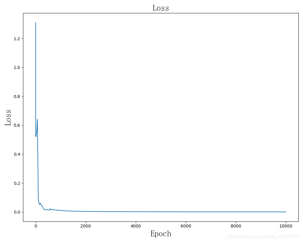
About weight initialization
Analysis of convergence rate of different initialization methods :
The learning rate is 0.01. The place to modify initialization is here :

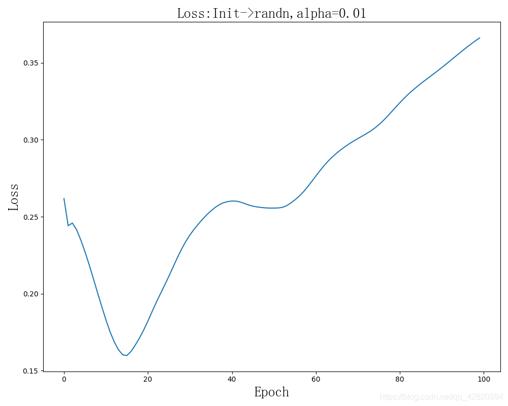
It seems that sometimes Loss The situation of increase , But random , It is related to initialization value and learning rate .
The final result of the first picture :epoch:99,loss:0.068638,accrucy : 0.903309

The effect is very poor .
epoch:99,loss:0.129023,accrucy : 0.307653

The effect was poor once , I want to boldly infer that the effect of such initialization is very poor , But this is unscientific , I try to change the learning rate to 0.1, The effect has been improved .
epoch:99,loss:0.129075,accrucy : 0.307653

epoch:99,loss:0.003670,accrucy : 0.767322

This initialization method is very bad , Although it decreases almost linearly , But the descent speed should not be too slow .
epoch:0,loss:4.500000,accrucy : 0.103413
epoch:12,loss:4.500000,accrucy : 0.103413
epoch:13,loss:4.500000,accrucy : 0.103930
epoch:499,loss:4.500000,accrucy : 0.105481
notes : bias b The way of initialization has little effect on convergence , This reader can try it by himself .
Why do different initialization converge at different speeds ?
To be continued ~
On the loss function
To be continued ~
About my feelings
The number of neurons in the hidden layer is not the more the better , I used to PyTroch I have tried to train a network similar to this one , Input layer , The output layer is the same as this neural network , At first, the hidden layer has 64 and 24 Neurons , The effect is good , But I try to change the number of neurons in the hidden layer to make it more , The effect is not good , And because of The amount of computation increases , The iteration speed is greatly reduced .
From the above experimental results, it seems that it is better to use the random value of standard normal distribution when initializing the weight , But that's why it's worth continuing to learn . Besides, it seems biased b The way of initialization has little effect on convergence , This reader can try it by himself .
About learning neural networks , If you think in terms of pragmatism , Then maybe you just need to understand the algorithm in the field of machine learning , Just learn to use the framework . But this is just useful .
If you want to study these networks , Try to improve its accuracy 、 Convergence rate 、 Forecast speed 、 Memory footprint 、 Complexity And so on , So as to create a new structure 、 Versatile structure 、 Structures that can be combined and so on need to have a deep understanding of them , Instead of just using the skin of a frame . Secondly, the learning process cannot be swallowed , Step by step , Focus on practice, summary and understanding .
About deceptive Neural Networks , Neural network vulnerability
appendix
Article resources
Handwritten digit recognition fully connected neural network teaching Demo: take digits.zip Unzip to net.py, After installing the environment, it can run .
git clone https://github.com/MisakaMikoto128/FCNNeuralNetworkDemoForHandwrittenDigits.git
Reference resources
[1] Neural network derivation
[2] Common loss function (loss function) summary
[3] Matrix derivation ( On )
[4] Matrix derivation ( Next )
[5] Xiaobai can understand it softmax Detailed explanation
Link failure Call I .
github:https://github.com/MisakaMikoto128
Personal website
边栏推荐
- 用指针访问一维数组
- Multi merchant mall system function disassembly Lecture 10 - platform end commodity units
- json.dumps()函数解析
- "Statistical learning methods (2nd Edition)" Li Hang Chapter 15 singular value decomposition SVD mind map notes and after-school exercise answers (detailed steps) SVD matrix singular value Chapter 15
- STM32 standard peripheral Library (Standard Library) official website download method, with 2021 latest standard firmware library download link
- PLSQL query data garbled
- Signals and systems: Hilbert transform
- CRC-16 Modbus代码
- C语言链表(创建、遍历、释放、查找、删除、插入一个节点、排序,逆序)
- 数据归一化
猜你喜欢

学习率优化策略

Positional argument after keyword argument
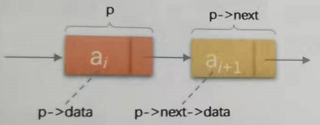
C语言链表(创建、遍历、释放、查找、删除、插入一个节点、排序,逆序)

Multi merchant mall system function disassembly lecture 09 - platform end commodity brands
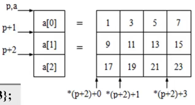
用指针访问二维数组

《统计学习方法(第2版)》李航 第22章 无监督学习方法总结 思维导图笔记

谷歌/火狐浏览器管理后台新增账号时用户名密码自动填入的问题

synergy局域网实现多主机共享键鼠(amd、arm)

《机器学习》(周志华) 第3章 线性模型 学习心得 笔记
Multi merchant mall system function disassembly lecture 13 - platform side member management
随机推荐
学习率优化策略
《统计学习方法(第2版)》李航 第十三章 无监督学习概论 思维导图笔记
Xshell远程访问工具
【树莓派4B】七、远程登录树莓派的方法总结XShell,PuTTY,vncServer,Xrdp
tensorflow和pytorch框架的安装以及cuda踩坑记录
Multi merchant mall system function disassembly Lecture 10 - platform end commodity units
[activiti] activiti process engine configuration class
世界坐标系、相机坐标系和图像坐标系的转换
数据归一化
[MYCAT] Introduction to MYCAT
Two architectures of data integration: ELT and ETL
Qt char型转QString型 16进制与char型 转 16进制整型
json.dumps()函数解析
[MYCAT] MYCAT configuration file
STM32 DSP库MDK VC5\VC6编译错误: 256, (const float64_t *)twiddleCoefF64_256, armBitRevIndexTableF64_256,
STM32 DSP library MDK vc5\vc6 compilation error: 256, (const float64_t *) twiddlecoeff64_ 256, armBitRevIndexTableF64_ 256,
测试数据增强后标签和数据集是否对应
对ArrayList<ArrayList<Double>>排序
【深度学习】手把手教你写“手写数字识别神经网络“,不使用任何框架,纯Numpy
信号与系统:希尔伯特变换