Review and analysis of noodle dishes

NetEase cloud music 《 Noodles and vegetables 》 Comment analysis

1、《 Noodles and vegetables 》 Basic analysis of music criticism

1.1、 Music background

《 Noodles and vegetables 》 This pure music is written by Lin Shengxiang Singing , It's the power supply 《 Great Buddha Plath 》 Music for ,《 Noodles and vegetables 》 It is undoubtedly the best score of the Great Buddha Plath , When the hero finds out the boss' secret, he never says much until his friend dies, and even his friend doesn't really understand , Just like this score, it's easy and pleasant, but with ridicule , This ridicule is not to laugh at others, but to laugh at your own face, cowardice and indifference to your friends , I found the secret of murder and found that my friend died inexplicably, but I didn't dare to say or do anything. I thought that others were bad people , Only choose to be a cowardly and indifferent person , Finally, I still don't care about anything and continue to live an ordinary and boring life, as if everything is a comedy, whistling and humming, and continue to be confused , Finally, the knocking of the Giant Buddha is nothing more than asking the protagonist what we are doing and what we are doing ！

1.2、 User profile analysis

1.2.1、 High frequency users are mainly after listening to music , I have regrets about the number of people

After analysis , by 【NO__EXCUSE_ 】 Of users commented 118 Time , The second is 【tianleigungunau】 Commented on 81 Time ,【 Please add some ice to coke 】 Commented on 57 Time , These users are mainly after listening to music , Expressed feelings , Said to go out often , For fun , Don't just be busy with work ！

1.2.2、 super 4 Adult users have no grade information

After analysis , nothing vip The number of level users is the most , the height is 7724 individual , The second is 6 and 5 Class users , There were 3131,2522 individual , It shows that high-level users are also more likely to comment

1.2.3、 The account number has been cancelled and the bottle of water is my favorite 、freechoice It depends heavily on the platform

After analysis ,【 Account has been cancelled 】 The cumulative number of songs ranked first , I have listened to it in total 280446 Time , The second is 【 I cherish the bottle of water 、】 Second place , I have listened to it in total 269442 Time ,【freechoice】 Ranked No 3, I have listened to it in total 133169 Time ,

1.2.4、 super 5 Adult users are not used to filling in regional information

After analysis , The number of users in unknown regions is as high as 9437 individual , Comment users are mainly distributed in coastal areas and southwest Sichuan

1.2.5、 super 8 Adult users are unwilling to disclose age information

After analysis ,89.47% The comment user of did not fill in the date of birth , In the group that revealed the date of birth ,18-24 Year old users account for the total 7.49%,18 Users under the age of account for the total 5.73%, Most of them are young people

1.2.5、 Commenting users have new views on life , Encourage yourself to relax properly , Cheer up , Avoid being confused

After analysis , Before the word frequency appears 10 It's about ambition , Power Supply , come on. , song , life , life , Belly wealth , Buddha , No, , Plath . Some of these words are movie titles , Or movie characters , Throughout the film ,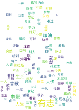

2、 At the end of the article, the code

• notes ： This article is written through jupyter notebook complete , It is also recommended that you use jupyter notebook Complete the exercises in the text

2.1、 Data base

# Import package 
import pandas as pd
import numpy as np
import os

# Reading data 
path = os.getcwd()+os.path.join("\\"," Comments on noodle dishes .xlsx")
df = pd.read_excel(path)
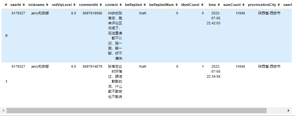
df.head(2)

data = df.copy()
df.info()

df.describe()

# View data shapes 
df.shape
#(23160, 12)

# View column headers 
df.columns

2.2、 Data processing and Visualization

2.2.1、 Comment frequency Top10 User information

# Import data visualization package 
from pyecharts import options as opts
from pyecharts.charts import Bar
from pyecharts.charts import Line
from pyecharts.charts import Map
from pyecharts.charts import Pie
from pyecharts.render import make_snapshot
from pyecharts.render import make_snapshot
from snapshot_selenium import snapshot

# Process user name 
def dealUserName(df,df1):
    userName = []
    for id in df1:
        index = df['userId'].tolist().index(id)
        userName.append(df['nickname'][index])
    return userName
    
# Count the number of comments per user , see Top10 Who are the users 
userReviewCount = df.groupby(by='userId')['userId'].count().sort_values(ascending=False)[:10]
userReviewCount = userReviewCount.sort_values(ascending=True)
userName = dealUserName(df,userReviewCount.index.tolist())

bar = (
    Bar(init_opts=opts.InitOpts(width="1500px",height="800px"))
    .add_xaxis(userName)
    .add_yaxis(" Comment frequency ", userReviewCount.tolist(),label_opts=opts.LabelOpts(position="right"),
              color = "#8CBD30")
    .reversal_axis()
    .set_global_opts(title_opts=opts.TitleOpts(title=" Number of user comments Top10", subtitle=" Data sources ： Yi Yun ",
                                               pos_left="center"),
                     xaxis_opts=opts.AxisOpts(name=" comments "),  #  add to X Axis title 
                     yaxis_opts=opts.AxisOpts(name=" user name "),  #  add to Y Axis title 
                     legend_opts=opts.LegendOpts(is_show=False))  #  Don't show legend 

)
bar.render_notebook()

2.2.2、 Different vip Level users

#vip Level users 
df['redVipLevel'] = df['redVipLevel'].apply(lambda x:x if str(x)!='nan' else 0)
vipUserLevelCount = df.drop_duplicates(subset= ['userId']).groupby(by='redVipLevel')['redVipLevel'].count()
bar = (
    Bar(init_opts=opts.InitOpts(width="1500px",height="800px"))
    .add_xaxis(vipUserLevelCount.index.tolist())
    .add_yaxis("",vipUserLevelCount.tolist(),label_opts=opts.LabelOpts(position="right"),
              color = "#8CBD30")
    .reversal_axis()
    .set_global_opts(title_opts=opts.TitleOpts(title=" Different vip Level users ", subtitle=" Data sources ： Yi Yun ",
                                               pos_left="center"),
                     xaxis_opts=opts.AxisOpts(name=" The number of users "),  #  add to X Axis title 
                     yaxis_opts=opts.AxisOpts(name="vip Grade "),  #  add to Y Axis title 
                     legend_opts=opts.LegendOpts(is_show=False))  #  Don't show legend 

)
bar.render_notebook()

2.2.3、 Cumulative number of songs Top10 User information

# Cumulative number of songs Top10 user 
sumListenSongCount = df[['userId','sumCount']].drop_duplicates(subset= ['userId']).sort_values(by='sumCount',ascending=False)[:10]
sumListenSongCount = sumListenSongCount.sort_values(by='sumCount',ascending=True)
# sumListenSongCount['userId']
userName = dealUserName(df,sumListenSongCount['userId'])
bar = (
    Bar(init_opts=opts.InitOpts(width="1500px",height="800px"))
    .add_xaxis(userName)
    .add_yaxis("",sumListenSongCount['sumCount'].tolist(),label_opts=opts.LabelOpts(position="right"),
              color = "#8CBD30")
    .reversal_axis()
    .set_global_opts(title_opts=opts.TitleOpts(title=" Users listen to songs in total Top10", subtitle=" Data sources ： Yi Yun ",
                                               pos_left="center"),
                     xaxis_opts=opts.AxisOpts(name=" Cumulative number of songs "),  #  add to X Axis title 
                     yaxis_opts=opts.AxisOpts(name=" user name "),  #  add to Y Axis title 
                     legend_opts=opts.LegendOpts(is_show=False))  #  Don't show legend 

)
bar.render_notebook()

2.2.4、 Cumulative number of songs Top10 User information

# Regional distribution of users 
def dealProvince(x:str)->str:
    
    if x == 'nan':
        x = " Unknown "
    else:
        if "-" in x:
            x = x.split('-')[0]
        else:
            x = x
    if ' province ' in x:
        x = x.replace(' province ', '')
    elif ' City ' in x:
        x = x.replace(' City ', '')
    elif ' Special Administrative Region ' in x:
        x = x.replace(' Special Administrative Region ', '')
    elif ' The Uygur Autonomous Region ' in x:
        x = x.replace(' The Uygur Autonomous Region ', '')
    elif ' The Hui Autonomous Region ' in x:
        x = x.replace(' The Hui Autonomous Region ', '')
    elif ' Zhuang Autonomous Region ' in x:
        x = x.replace(' Zhuang Autonomous Region ', '')
    elif ' Autonomous region ' in x:
        x = x.replace(' Autonomous region ', '')
    else:
        x = x
    return x

def dealProvinceRate(Series):
    provinceDict = {}
    sum = 0
    for index,s in enumerate(Series.index.tolist()):
        if s == " Unknown ":
            provinceDict[" Unknown "] = Series.tolist()[index]
        elif s == " overseas ":
             provinceDict[" overseas "] = Series.tolist()[index]
        else:
            sum += Series.tolist()[index]
    provinceDict[" At home "] = sum
    return provinceDict
    
userAreaCount = df.drop_duplicates(subset= ['userId'])['provinceAndCity'].apply(lambda x:dealProvince(str(x)))
userAreaCount = userAreaCount.groupby(by=userAreaCount).count().sort_values(ascending=False)
provinceDict = dealProvinceRate(userAreaCount)
pie = (
    Pie()
    .add(
        "",
        [list(z) for z in zip(provinceDict.keys(),provinceDict.values())],
        radius=["40%", "75%"],
    )
    .set_colors(["#8CBD30","#479DE3","#045F96"])
    .set_global_opts(
        title_opts=opts.TitleOpts(title=" Proportion of user area ",subtitle=" Data sources ： Yi Yun ",pos_left="center"),
        legend_opts=opts.LegendOpts(orient="vertical", pos_top="15%", pos_left="15%"),
    )
    .set_series_opts(label_opts=opts.LabelOpts(formatter="{b}: {c}"))
)
pie.render_notebook()

2.2.5、 Users at home and abroad

p_data = [list(z) for z in zip(userAreaCount.index.tolist(),userAreaCount.tolist())]
map = (
 Map(init_opts=opts.InitOpts(width="1500px",height="800px"))
 .add(' The number of users ',p_data,'china',is_map_symbol_show=False,itemstyle_opts={
    "normal":{"areaColor":"white","borderColor":""}
})
 .set_series_opts(label_opts=opts.LabelOpts(is_show=True))
 .set_global_opts(title_opts=opts.TitleOpts(title = ''),
     visualmap_opts=opts.VisualMapOpts(
          max_=9999,
          is_piecewise=True,
          pos_left='30%',
          pos_bottom='10%',
          pieces=[
                {"max": 99, "min": 0, "label": "100 following ","color":"#D9D9D9"},
              {"max": 200, "min":100, "label": "100-200","color":"#8CBD30"},
              {"max": 300, "min": 201, "label": "201-300","color":"#479DE3"},
              {"max": 400, "min": 301, "label": "301-400","color":"#045F96"},
              {"max": 9999, "min":401, "label": "400 above ", "color":"#FFC000"}
          ]
        )
    ,
    legend_opts = opts.LegendOpts(is_show=False)
   )
 ) 
map.render_notebook()

2.2.6、 The situation of domestic users in various provinces

p_data = [list(z) for z in zip(userAreaCount.index.tolist(),userAreaCount.tolist())]
map = (
 Map(init_opts=opts.InitOpts(width="1500px",height="800px"))
 .add(' The number of users ',p_data,'china',is_map_symbol_show=False,itemstyle_opts={
    "normal":{"areaColor":"white","borderColor":""}
})
 .set_series_opts(label_opts=opts.LabelOpts(is_show=True))
 .set_global_opts(title_opts=opts.TitleOpts(title = ''),
     visualmap_opts=opts.VisualMapOpts(
          max_=9999,
          is_piecewise=True,
          pos_left='30%',
          pos_bottom='10%',
          pieces=[
                {"max": 99, "min": 0, "label": "100 following ","color":"#D9D9D9"},
              {"max": 200, "min":100, "label": "100-200","color":"#8CBD30"},
              {"max": 300, "min": 201, "label": "201-300","color":"#479DE3"},
              {"max": 400, "min": 301, "label": "301-400","color":"#045F96"},
              {"max": 9999, "min":401, "label": "400 above ", "color":"#FFC000"}
          ]
        )
    ,
    legend_opts = opts.LegendOpts(is_show=False)
   )
 ) 
 map.render_notebook()

2.2.7、 Age distribution of users

# User age distribution 
from datetime import datetime
def dealUserAge(x)->str:
    if type(x) == pd._libs.tslibs.nattype.NaTType:
        x = " Unknown "
    else:
        x = (pd.to_datetime("2022-07-17")-x)/pd.Timedelta('365 days')
        if x<18:
            x = "18 Under the age of "
        elif x>=18 and x<=24:
            x = "16-24 year "
        elif x>=25 and x<=30:
             x = "25-30 year "
        elif x>=31 and x<=35:
             x = "31-35 year "
        else:
            x = "35 Years of age or older "
    return x


userAgeArea= df.drop_duplicates(subset= ['userId'])['userBirthDate']
userAgeArea = pd.to_datetime(userAgeArea,errors='coerce').apply(lambda x:dealUserAge(x))
userAgeArea = userAgeArea.groupby(by=userAgeArea).count().sort_values(ascending=False)
pie = (
    Pie()
    .add(
        "",
        [list(z) for z in zip(userAgeArea.index,[str(round(i/sum(userAgeArea),4)) for i in userAgeArea])],
        radius=["20%", "55%"],
    )
    .set_colors(["#FFC000","#8CBD30","#479DE3","#00ffff","#045F96","#D9D9D9"])
    .set_global_opts(
        title_opts=opts.TitleOpts(title=" The age proportion of users ",subtitle=" Data sources ： Yi Yun ",pos_left="center"),
        legend_opts=opts.LegendOpts(orient="vertical", pos_top="15%", pos_left="15%"),
    )
    .set_series_opts(label_opts=opts.LabelOpts(formatter="{b}: {d}%"))
)
pie.render_notebook()

2.2.8、 Basic analysis of user comments

# Import package 
import matplotlib.pyplot as plt
from wordcloud import WordCloud,ImageColorGenerator
%matplotlib inline
from PIL import Image
from imageio import imread
import jieba.analyse

#jieba participle 
def jieba_deal(data,k):
    content = data['content'].apply(jieba.lcut) # participle 
    stopword = [line.strip() for line in open(' Stoppage vocabulary of Harbin Institute of Technology .txt','r',encoding='utf-8').readlines()]  # Read stop words 
    content_list = []
    # Remove useless words 
    for text in content:
        for word in text:
            if word not in stopword:
                content_list.append(word)
    _content = ' '.join(content_list) # utilize join Methods use spaces to splice them 
    keywords = jieba.analyse.extract_tags(_content,topK=k,withWeight=True,allowPOS=()) # Extract the one with the highest weight 100 word 
    return keywords
jieba_deal(df,100)

keywords = jieba_deal(df,100)
keywords_dict = {} # Form a dictionary 
for keyword in keywords:
    keywords_dict[keyword[0]] = int(keyword[1]*10000)
graph = np.array(Image.open(' Buddha .png'))  # Read the target image to make the word cloud 

wc = WordCloud(font_path = 'simhei.ttf',      #  Set the font format , If you do not set the display of Chinese 
                          background_color="white",      #  Set the background color 
                          max_font_size=100,     #  Set font maximum 
                          mask = graph,
                          random_state=100,  #  Set how many randomly generated states there are , That's how many color schemes there are 
                          relative_scaling=.5
                          ).fit_words(keywords_dict) #word For dictionary format 
# image_corlors = ImageColorGenerator(graph)
plt.figure(figsize = [24,15])  # Picture size 
plt.imshow(wc)  
plt.axis('off')
plt.show() #  Display images 

3、 summary

This paper uses the data obtained python Carry out simple character portraits and word cloud analysis , It aims to understand the basic characteristics of comment users , There are still many deficiencies in the article , I hope you will correct me ！！！