当前位置:网站首页>ESWC 2018 | r-gcn: relational data modeling based on graph convolution network
ESWC 2018 | r-gcn: relational data modeling based on graph convolution network
2022-07-25 04:35:00 【Cyril_ KI】
Catalog
Preface

subject : Modeling Relational Data with Graph Convolutional Networks
meeting : Extended Semantic Web Conference, 2018
Address of thesis :Modeling Relational Data with Graph Convolutional Networks
This article is GCN The author of Kipf Following GCN The latter work ,GCN There are two obvious problems :
- Can only deal with undirected graphs
- Can only deal with homogeneous graphs , That is, only edges of the same type can be processed .
R-GCN As GCN The follow-up work of , Its main contribution is to GCN It is introduced into multi relation heterogeneous graph , in other words R-GCN When updating node features, we can consider the characteristics of different types of edge nodes .
1. Graph convolution network
Definition of terms : The Internet G = ( V , E , R ) G=(\mathcal{V},\mathcal{E}, \mathcal{R}) G=(V,E,R), Where nodes v i ∈ V v_i \in \mathcal{V} vi∈V, edge ( v i , r , v j ) ∈ E (v_i,r,v_j) \in \mathcal{E} (vi,r,vj)∈E, among r ∈ R r \in \mathcal{R} r∈R Indicates the type of edge .
GCN and R-GCN Both use graph convolution to update node status , The two can be unified with the following framework :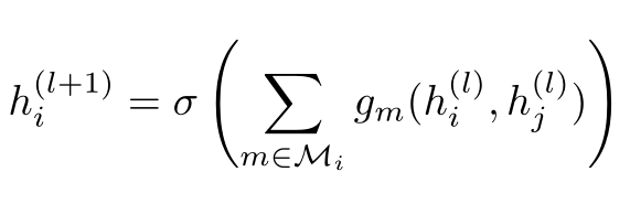
here h i ( l ) h_i^{(l)} hi(l) Representation node v i v_i vi The first l l l The hidden state of a layer , g m ( . , . ) g_m(.,.) gm(.,.) It can be understood as the message function mentioned in the previous article , M i \mathcal{M}_i Mi Refers to the node v i v_i vi Incoming message collection of , σ \sigma σ Is the activation function .
about GCN Speaking of , g m ( . , . ) g_m(.,.) gm(.,.) It means multiplying the characteristics of neighbor nodes by the normalized weight coefficient , here GCN The type information of nodes is not considered , Because all nodes belong to the same type .
about R-GCN Speaking of , A key problem is how to consider the differences between different types of nodes in the convolution process , That is, how to interact among multiple relationships . For different types of relationships in the diagram ,R-GCN Here's how :
among :
- N i r \mathcal{N}_i^r Nir: node v i v_i vi The relationship is r r r Set of neighbor nodes . For example, for a reference network , The relationship between the author node and other nodes may be “ The author writes a thesis ”、“ The author belongs to an organization ” wait .
- c i , r c_i,r ci,r Is a normalization coefficient , It can be set as a learnable parameter or a constant , for example ∣ N i r ∣ |\mathcal{N}_i^r| ∣Nir∣.
- W r ( l ) W_r^{(l)} Wr(l) Is a linear transformation function , Observation subscript r r r We can know , Each type of relationship has its own linear function , They are responsible for transforming the characteristics of neighbor nodes on the edge of the corresponding relationship .
By observing the above formula, we can find ,R-GCN After aggregating the node characteristics of different relationships , You also need to add the characteristics of your own nodes , Finally, an activation function is used to get the updated node characteristics .
R-GCN And GCN The big difference is this R-GCN Several linear transformation functions are introduced to transform various types of relational nodes , and GCN There is only one type of relationship in , That is, there is only one linear transformation function .
R-GCN The calculation diagram of single node update in is shown below :
The red node indicates the node to be updated , The dark blue node indicates the neighbor node of the node to be updated , They are divided into different groups according to their relationships , At the same time, the nodes in each group are divided into internal relationship nodes and external relationship nodes according to the direction of the edge . The state of the dark blue node is transformed into a green node through the transformation function , Then gather together ( Due to the addition of self-loop, The characteristics of the red node itself are also taken into account ). Last , The aggregated features get the updated state of the red node through an activation function .
2. Regularization
R-GCN You need to specify a conversion function for each type of edge W W W, If a network has many kinds of relationships , that R-GCN The number of parameters in will also increase dramatically , Cause huge computational overhead .
To solve this problem , An intuitive idea is that conversion functions with different types of relationships share parameters , However, if the parameters are fully shared R-GCN Will degenerate into GCN. So , The author puts forward basis function decomposition, That is, basis function decomposition :
It can be seen from the decomposition formula of the basis function , Different relationships r r r The transformation function of is obtained by a linear combination , The first l l l Of transformation functions with different relationships in the layer V b ( l ) V_b^{(l)} Vb(l) identical , Just the combination coefficient a r b ( l ) a_{rb}^{(l)} arb(l) Different , This greatly reduces the number of parameters .
The author also puts forward block-diagonal decomposition, Block diagonal decomposition method . Specifically speaking, it is :
You can find , Each linear transformation function passes through a set of low dimensional matrices Q b r Q_{br} Qbr To define , namely :
Basis function decomposition can be regarded as a form of effective weight sharing between different relationship types , The block diagonal decomposition can be regarded as the sparsity constraint on the weight matrix of each relationship type . The block diagonal decomposition structure encodes an intuition , That is, potential features can be divided into a set of variables , These variables are more closely coupled within groups than between groups . Both of these decompositions reduce highly multi relational data ( Such as the real knowledge base ) The number of parameters to learn .
3. experiment
3.1 Node classification
Node classification can be summarized as follows :
Simply put, by stacking multiple R-GCN Layer to get the vector representation of nodes , And then through softmax Function gets the output , Finally, the model parameters are updated by calculating the cross entropy loss function , This is the same as mentioned earlier GNN The node classification model is consistent .
The cross entropy loss function is defined as :
among Y \mathcal{Y} Y Is the index set of labeled nodes , h i k ( L ) h_{ik}^{(L)} hik(L) Representation node i i i Of the output of k k k term , t i k t_{ik} tik Indicates the true value of the corresponding tag .
Entities of the dataset used in the experiment 、 Relationship 、 edge 、 Labels and categories are as follows :
Baseline:RDF2Vec、Weisfeiler-Lehman kernels (WL) 、Feat( A manually designed feature extractor ).
experimental result :
You can find ,R-GCN stay MUTAG and BGS Didn't do the best , The explanation given by the author is :MUTAG and BGS There are many medium height nodes . In particular : Normalization constant of message aggregation from adjacent nodes 1 / c i , r 1/c_{i, r} 1/ci,r Fixed choice is part of the reason for this behavior , For height nodes , This can be particularly problematic . In the future work , A potential way to overcome this limitation is to introduce an attention mechanism , That is, use the attention weight of data dependence a i j , r a_{ij,r} aij,r Replace the normalization constant 1 / c i , r 1/c_{i, r} 1/ci,r.
3.2 Link prediction
For link prediction, please refer to my previous article :PyG build GCN Realize link prediction .
Link prediction model is divided into encoder and decoder , The encoder is R-GCN, That is, through R-GCN Encode the nodes to get a low dimensional vector representation , Then through the decoder DistMult That is, the score function gets the score between node vector pairs , Then the cross entropy loss function is obtained with the real sample , Finally, update the parameters .
Data sets :
experimental result :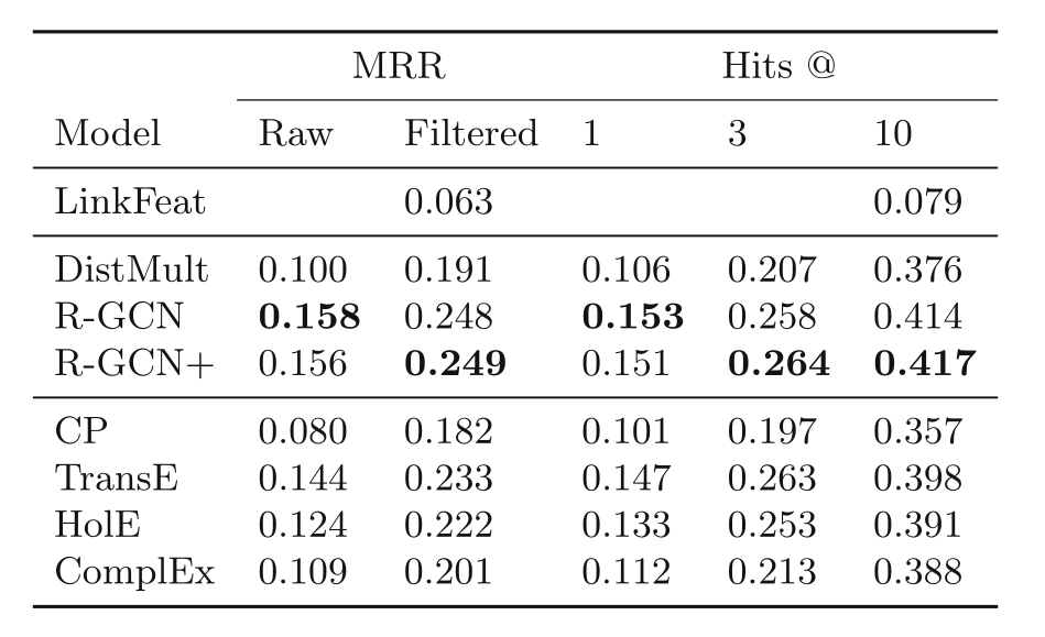
边栏推荐
- Mit.js: small event publishing and subscription library
- When the development of the meta universe begins to show more and more the style of the Internet, we need to be vigilant
- Network engineering case: integrated network design of CII company
- Aggregate payment meets the needs of various industries to access a variety of payments
- 市场是对的
- Analytic hierarchy process of MATLAB
- Only list the data of the specified field GetData ($table, '*', $where, $order)
- Math. Random, switch selection structure
- LVGL 8.2 Message box
- Construction of data center (I): background of the emergence of data center
猜你喜欢

Summary of UPR optimization suggestions of unity

【浅析STM32之GPIO寄存器(CRL/CRH)配置 】

暗黑王者|ZEGO 低照度图像增强技术解析

【基于stm32f103的SHT30温湿度显示】
Dark king | analysis of zego low illumination image enhancement technology

Attack and defense world ----- ics-05

MongoDB的安全认证详解

Interview required: how to design the seckill system?

5年经验的大厂测试/开发程序员,怎样突破技术瓶颈?大厂通病......
Open source summer interview | "after 00" PMC member Bai Zeping
随机推荐
Current characteristics of steering gear with great resistance
Source code | opencv DNN + yolov7 target detection
Opencv4.5.x+cuda11.0.x source code compilation and yolov5 acceleration tutorial!
Apple airpower was forced to cancel its launch two years after it was launched! Uncover the reason!
看问题的角度
When developing or debugging the IP direct scheme, it should be noted that the host value should be consistent with the direct IP
Burpsuite爆破之token值替换
读书的思考
Interview required: how to design the seckill system?
自然的状态最好
Open source summer interview | "after 00" PMC member Bai Zeping
开源之夏专访|“00 后” PMC member 白泽平
LVGL 8.2 Message box
The interviewer asked MySQL transactions, locks and mvcc at one go. I
GDT,LDT,GDTR,LDTR
Cannot make qopenglcontext current in a different thread: the solution to pyqt multithread crash
Application of AI in testing
etcd学习
Interpretation and download of the report | ink Tianlun July database industry report, be prepared for danger in times of safety, and safety first
Paper:《Peeking Inside the Black Box: Visualizing Statistical Learning with Plots of Individual Condi