In depth study paper reading target detection (VII) Chinese English Bilingual Edition: yolov4 optimal speed and accuracy of object detection

Abstract Abstract

  There are a huge number of features which are said to improve Convolutional Neural Network (CNN) accuracy. Practical testing of combinations of such features on large datasets, and theoretical justification of the result, is required. Some features operate on certain models exclusively and for certain problems exclusively, or only for smallscale datasets; while some features, such as batch-normalization and residual-connections, are applicable to the majority of models, tasks, and datasets. We assume that such universal features include WeightedResidual-Connections (WRC), Cross-Stage-Partial-connections (CSP), Cross mini-Batch Normalization (CmBN), Self-adversarial-training (SAT) and Mish-activation. We use new features: WRC, CSP, CmBN, SAT, Mish activation, Mosaic data augmentation, CmBN, DropBlock regularization, and CIoU loss, and combine some of them to achieve state-of-the-art results: 43.5% AP (65.7% AP50 ) for the MS COCO dataset at a real-time speed of ∼65 FPS on Tesla V100. Source code is at GitHub.

   There are a number of techniques to improve convolutional neural networks （CNN） The accuracy of the . Need to be in big The combination of this technique is actually tested under the data set , And need to theorize about the results Prove . Some techniques are used only on certain models and are specific to certain problems , Or only for small Large data sets ; And some skills , Such as batch normalization 、 Residual connection, etc , Apply to Most models 、 Tasks and datasets . We assume that this general technique includes weighted residuals Differential connection （Weighted-Residual-Connection,WRC）、 Across small batch connections (Cross-Stage-Partial-connection,CSP)、Cross mini-Batch Normalization （CmBN）、 Self confrontation training （Self-adversarial-training,SAT） and Mish Thrill Live functions . We use these new techniques in this article ：WRC、CSP、CmBN、SAT, Mish-activation,Mosaic data augmentation、CmBN、DropBlock Regular Hua He CIoU Loss , And a combination of these techniques , stay MS COCO The data set reaches the goal The best result before ：43.5% Of AP（65.7% AP50）, stay Tesla V100 Up to To about 65FPS. See source code ：GitHub

1. Introduction introduction

  The majority of CNN-based object detectors are largely applicable only for recommendation systems. For example, searching for free parking spaces via urban video cameras is executed by slow accurate models, whereas car collision warning is related to fast inaccurate models. Improving the real-time object detector accuracy enables using them not only for hint generating recommendation systems, but also for stand-alone process management and human input reduction. Real-time object detector operation on conventional Graphics Processing Units (GPU) allows their mass usage at an affordable price. The most accurate modern neural networks do not operate in real time and require large number of GPUs for training with a large mini-batch-size. We address such problems through creating a CNN that operates in real-time on a conventional GPU, and for which training requires only one conventional GPU.
   Most are based on CNN The target detectors are basically only applicable to the recommended system . example Such as ： Look for free parking spaces through city cameras , It is done by an accurate slow model , and The car collision warning needs to be provided by the fast 、 Low precision model completion . Improve the performance of real-time target detector precision , It can not only be used to prompt the generation of recommendation system , It can also be used for independent Process management and reduction of human input . Tradition GPU So that target detection can be carried out at an affordable price Grid operation . The most accurate modern neural networks do not run in real time , Requiring a lot of training GPU With big mini bacth size. Let's create a CNN To solve this problem problem , In traditional GPU Real time operation on , For these exercises, only one is needed Conventional GPU.
  The main goal of this work is designing a fast operating speed of an object detector in production systems and optimization for parallel computations, rather than the low computation volume theoretical indicator (BFLOP). We hope that the designed object can be easily trained and used. For example, anyone who uses a conventional GPU to train and test can achieve real-time, high quality, and convincing object detection results, as the YOLOv4 results shown in Figure 1. Our contributions are summarized as follows: 1. We develope an efficient and powerful object detection model. It makes everyone can use a 1080 Ti or 2080 Ti GPU to train a super fast and accurate object detector. 2. We verify the influence of state-of-the-art Bag-ofFreebies and Bagof-Specials methods of object detection during the detector training. 3. We modify state-of-the-art methods and make them more effecient and suitable for single GPU training, including CBN [89], PAN [49], SAM [85], etc.
   The main purpose of this research is to design a target that can run quickly in the production environment detector , And parallel computing optimization , It is not a theoretical index with low calculation amount （BFLOP）. We want the goal to be easy to train and use . for example , Anything that makes With tradition GPU People who train and test can achieve real-time 、 High-quality 、 Persuasive Force target detection results ,YOLOv4 The results are shown in the figure 1 Shown . Now our achievements are summarized as As follows ： 1. We built a fast 、 Powerful models , This makes it possible for everyone to use 1080 Ti or 2080 Ti GPU To train a super fast 、 Accurate target detector . 2. We have verified the most advanced Bag-of-Freebies and Bag-of-Specials Method Impact during target detection training . 3. We modified the most advanced method , Make it more efficient and suitable for single GPU Training , Include CBN[89]、PAN[49]、SAM[85] etc. .

2. Related work Related work

2.1. Object detection models Target detection model

  A modern detector is usually composed of two parts, a backbone which is pre-trained on ImageNet and a head which is used to predict classes and bounding boxes of objects. For those detectors running on GPU platform, their backbone could be VGG [68], ResNet [26], ResNeXt [86], or DenseNet [30]. For those detectors running on CPU platform, their backbone could be SqueezeNet [31], MobileNet [28, 66, 27, 74], or ShuffleNet [97, 53]. As to the head part, it is usually categorized into two kinds, i.e., one-stage object detector and two-stage object detector. The most representative two-stage object detector is the R-CNN [19] series, including fast R-CNN [18], faster R-CNN [64], R-FCN [9], and Libra RCNN [58]. It is also possible to make a two-stage object detector an anchorfree object detector, such as RepPoints [87]. As for one-stage object detector, the most representative models are YOLO [61, 62, 63], SSD [50], and RetinaNet [45]. In recent years, anchor-free one-stage object detectors are developed. The detectors of this sort are CenterNet [13], CornerNet [37, 38], FCOS [78], etc. Object detectors developed in recent years often insert some layers between backbone and head, and these layers are usually used to collect feature maps from different stages. We can call it the neck of an object detector. Usually, a neck is composed of several bottom-up paths and several top-down paths. Networks equipped with this mechanism include Feature Pyramid Network (FPN) [44], Path Aggregation Network (PAN) [49], BiFPN [77], and NAS-FPN [17]. In addition to the above models, some researchers put their emphasis on directly building a new backbone (DetNet [43], DetNAS [7]) or a new whole model (SpineNet [12], HitDetector [20]) for object detection.

   Modern target detectors usually consist of two parts ：ImageNet Pre trained backbone And are used to predict categories and BBOX The detector head. For those in GPU Detectors running on the platform , Its backbone It can be VGG[68],ResNet[26]、 ResNeXt[86]、 or DenseNet [30]. For those running on CPU Detection on the platform Device form , Their backbone It can be SqueezeNet[31]、MobileNet[28,66, 27,74], or ShuffleNet[97,53]. as for head part , It is usually divided into two categories ： That is, one stage （one-stage） And two stages （two-stage） The target detector . The most modern The representational two-stage detector is R-CNN[19] Series model , Include Fast R-CNN[18]、 Faster R-CNN[64]、R-FCN[9] and Libra R-CNN[58]. It can also be done in two stages Not used in standard detector anchor The target detector , Such as RepPoints[87]. For first order Segment detector , The most representative ones are YOLO[61、62、63]、SSD[50] and RetinaNet[45]. in recent years , Also developed many do not use anchor The first stage goal of detector . This type of detector has CenterNet[13]、CornerNet[37,38]、FCOS[78] etc. . In recent years, the development of detectors is often in backbone and head Insert some layers between , These layers are used to collect characteristic maps of different stages . We can call it the detector neck. Usually neck There are several bottom-up or top-down pathways （paths） form . Networks with this structure include Feature Pyramid Network (FPN)[44]、Path Aggregation（PAN）[49]、BiFPN[77] and NAS-FPN[17]. In addition to the above model , Some researchers focus on direct reconstruction backbone（DetNet[43]、DetNAS[7]） Or rebuild the entire model （SpineNet[12]、HitDetector[20]), And used for target detection Test task .

  To sum up, an ordinary object detector is composed of several parts:

   Sum up , Generally, the target detection model consists of the following parts ：

2.2. Bag of freebies

  Usually, a conventional object detector is trained offline. Therefore, researchers always like to take this advantage and develop better training methods which can make the object detector receive better accuracy without increasing the inference cost. We call these methods that only change the training strategy or only increase the training cost as “bag of freebies.” What is often adopted by object detection methods and meets the definition of bag of freebies is data augmentation. The purpose of data augmentation is to increase the variability of the input images, so that the designed object detection model has higher robustness to the images obtained from different environments. For examples, photometric distortions and geometric distortions are two commonly used data augmentation method and they definitely benefit the object detection task. In dealing with photometric distortion, we adjust the brightness, contrast, hue, saturation, and noise of an image. For geometric distortion, we add random scaling, cropping, flipping, and rotating.

   Usually , The traditional training of target detector is carried out offline . therefore , Researchers always like to use the benefits of pure training to study better training methods , bring The target detector achieves better accuracy without increasing the test cost . We put these The method that only needs to change the training strategy or only increase the training cost is called bag of freebies. Objective Data enhancement is often used and meets this definition . The purpose of data enhancement is Increase the diversity of input images , Thus, the designed target detection model can be applied to different environments The image of has high robustness . such as photometric distortions and geometric distortions Are two commonly used data enhancement methods , They must be good for the detection task Situated . Use photometric distortions when , We adjust the brightness of the image 、 Contrast 、 tonal 、 Saturation and noise . Use geometric distortions when , We add... To the image Random scaling 、 tailoring 、 Flip and rotate .

  The data augmentation methods mentioned above are all pixel-wise adjustments, and all original pixel information in the adjusted area is retained. In addition, some researchers engaged in data augmentation put their emphasis on simulating object occlusion issues. They have achieved good results in image classification and object detection. For example, random erase [100] and CutOut [11] can randomly select the rectangle region in an image and fill in a random or complementary value of zero. As for hide-and-seek [69] and grid mask [6], they randomly or evenly select multiple rectangle regions in an image and replace them to all zeros. If similar concepts are applied to feature maps, there are DropOut [71], DropConnect [80], and DropBlock [16] methods. In addition, some researchers have proposed the methods of using multiple images together to perform data augmentation. For example, MixUp [92] uses two images to multiply and superimpose with different coefficient ratios, and then adjusts the label with these superimposed ratios. As for CutMix [91], it is to cover the cropped image to rectangle region of other images, and adjusts the label according to the size of the mix area. In addition to the above mentioned methods, style transfer GAN [15] is also used for data augmentation, and such usage can effectively reduce the texture bias learned by CNN.

   The data enhancement methods mentioned above are all pixel by pixel adjustment , And adjust the area The original pixel information will be preserved . Besides , Some research on data enhancement The researchers focus on the problem of simulating target occlusion . They are in image classification and object detection Got good results . for example , Random erase [100] and CutOut[11] The graph can be selected randomly Rectangular area in image , And fill in random values or complementary values of zero . as for hide-and-seek [69] and grid mask [6], They randomly or evenly select multiple rectangular regions in the image , and Replace all its pixel values with zero values . If a similar concept is applied to a feature graph , Just yes DropOut[71]、DropConnect[80] and DropBlock[16] Method . Besides , Youyan Researchers have proposed a method of data enhancement by putting multiple images together . for example , MixUp[92] Multiply and superimpose the two images with different coefficients , And according to the stacking ratio For example, adjust the label . about CutMix[91], It overwrites the cropped image to other images The rectangular area of , And adjust the label according to the size of the mixing area . In addition to the methods mentioned above , Network migration GAN[15] It is also often used for data enhancement , This method can effectively reduce CNN Learned texture deviation .
  Different from the various approaches proposed above, some other bag of freebies methods are dedicated to solving the problem that the semantic distribution in the dataset may have bias. In dealing with the problem of semantic distribution bias, a very important issue is that there is a problem of data imbalance between different classes, and this problem is often solved by hard negative example mining [72] or online hard example mining [67] in two-stage object detector. But the example mining method is not applicable to one-stage object detector, because this kind of detector belongs to the dense prediction architecture. Therefore Lin et al. [45] proposed focal loss to deal with the problem of data imbalance existing between various classes. Another very important issue is that it is difficult to express the relationship of the degree of association between different categories with the one-hot hard representation. This representation scheme is often used when executing labeling. The label smoothing proposed in [73] is to convert hard label into soft label for training, which can make model more robust. In order to obtain a better soft label, Islam et al. [33] introduced the concept of knowledge distillation to design the label refinement network.
   Different from the various methods proposed above , Others Bag of freebies The method is Specifically solve the problem of semantic distribution in data sets that may have deviation . In dealing with semantic distribution deviation On the issue of , A very important problem is the data imbalance between different categories , And two The stage detector usually handles this problem by hard negative example mining [72] or online hard example mining [67]. but example mining method Do not apply Target detector in one stage , Because this detector is a dense prediction Architecture . therefore , Linet al.[45] Put forward focal loss Solve the problem of data imbalance . Another very important The problem is ,one-hot Coding is difficult to express the degree of association between classes . This representation is Law （one-hot） It is usually used in labeling . stay [73] Proposed in label smoothing The scheme is to transform hard tags into soft tags for training , It can make the model more Robust . In order to get better soft tags ,Islam etc. [33] Introduce the concept of knowledge distillation And used to design label refinement network .
  The last bag of freebies is the objective function of Bounding Box (BBox) regression. The traditional object detector usually uses Mean Square Error (MSE) to directly perform regression on the center point coordinates and height and width of the BBox, i.e., {xcenter, ycenter, w, h} , or the upper left point and the lower right point, i.e., {xtop_left, ytop_left, xbottom_right, ybottom_right}. As for anchor-based method, it is to estimate the corresponding offset, for example { x center offset , y center offset , w offset , h offset } and { x top left offset , y top left offset , x bottom right offset , y bottom right offset } . However, to directly estimate the coordinate values of each point of the BBox is to treat these points as independent variables, but in fact does not consider the integrity of the object itself. In order to make this issue processed better, some researchers recently proposed IoU loss [90], which puts the coverage of predicted BBox area and ground truth BBox area into consideration. The IoU loss computing process will trigger the calculation of the four coordinate points of the BBox by executing IoU with the ground truth, and then connecting the generated results into a whole code. Because IoU is a scale invariant representation, it can solve the problem that when traditional methods calculate the l1 or l2 loss of { x, y, w, h } , the loss will increase with the scale. Recently, some researchers have continued to improve IoU loss. For example, GIoU loss [65] is to include the shape and orientation of object in addition to the coverage area. They proposed to find the smallest area BBox that can simultaneously cover the predicted BBox and ground truth BBox, and use this BBox as the denominator to replace the denominator originally used in IoU loss. As for DIoU loss [99], it additionally considers the distance of the center of an object, and CIoU loss [99], on the other hand simultaneously considers the overlapping area, the distance between center points, and the aspect ratio. CIoU can achieve better convergence speed and accuracy on the BBox regression problem.
   the last one bag of freebies It's a bounding box (BBox) The objective function of regression . testing The device usually uses MSE Loss function pair BBOX The center point and width and height of , for example {xcenter, ycenter, w, h}, Or regression prediction of the upper left corner and the lower right corner , for example {xtop_left, ytop_left, xbottom_right, ybottom_right}. Based on anchor Methods , It will Estimate the corresponding offset , for example { x center offset , y center offset , w offset , h offset } and { x top left offset , y top left offset , x bottom right offset , y bottom right offset }. however , If you want to estimate directly BBOX Coordinate value of each point , Take these points as independent variables , But in fact, the integrity of the object itself is not considered . by This makes this problem better solved , Some researchers recently proposed IoU Loss [90], It takes into account the forecast BBox Area and ground truth BBox Coverage of area . IoU The loss calculation process will calculate the difference between the predicted value and the real value IoU, And then what will be generated The results are linked into a whole code , Finally, through calculation BBox Four coordinate values of . because IOU Is a scale independent representation , It can be solved when the traditional method calculates {x, y,w,h} Of l1 or l2 When it's lost , The problem that the loss will increase with the increase of scale . most near , Some researchers continue to improve IOU Loss . for example GIoU Loss [65] In addition to coverage The product also takes into account the shape and direction of the object . They suggest finding ways to cover predictions at the same time BBOX and True value BBox The smallest area of BBOX, And use this BBox As the denominator and replace The original IoU Denominator of loss . as for DIoU Loss [99], It also includes considering objects The distance from the center , On the other hand CIoU Loss [99] Taking into account the overlapping area and the center point The distance between them and the aspect ratio .CIoU Can be in BBox On the issue of regression The convergence rate and accuracy of .

2.3. Bag of specials

  For those plugin modules and post-processing methods that only increase the inference cost by a small amount but can significantly improve the accuracy of object detection, we call them “bag of specials”. Generally speaking, these plugin modules are for enhancing certain attributes in a model, such as enlarging receptive field, introducing attention mechanism, or strengthening feature integration capability, etc., and post-processing is a method for screening model prediction results.
   For those insert modules and post-processing methods that only add a small amount of reasoning cost , However, it can significantly improve the accuracy of target detection , We call it “Bag of specials”. One In general , These plug-in modules are used to enhance certain properties of the model , Such as expanding the receptive field 、 Introduce attention mechanism or enhance feature integration ability , Post processing is a screening model pre - processing Test result method .
  Common modules that can be used to enhance receptive field are SPP [25], ASPP [5], and RFB [47]. The SPP module was originated from Spatial Pyramid Matching (SPM) [39], and SPMs original method was to split feature map into several d × d equal blocks, where d can be { 1, 2, 3, … } , thus forming spatial pyramid, and then extracting bag-of-word features. SPP integrates SPM into CNN and use max-pooling operation instead of bag-of-word operation. Since the SPP module proposed by He et al. [25] will output one dimensional feature vector, it is infeasible to be applied in Fully Convolutional Network (FCN). Thus in the design of YOLOv3 [63], Redmon and Farhadi improve SPP module to the concatenation of max-pooling outputs with kernel size k × k, where k = { 1, 5, 9, 13 } , and stride equals to 1. Under this design, a relatively large k × k maxpooling effectively increase the receptive field of backbone feature. After adding the improved version of SPP module, YOLOv3-608 upgrades AP 50 by 2.7% on the MS COCO object detection task at the cost of 0.5% extra computation. The difference in operation between ASPP [5] module and improved SPP module is mainly from the original k×k kernel size, max-pooling of stride equals to 1 to several 3 × 3 kernel size, dilated ratio equals to k, and stride equals to 1 in dilated convolution operation. RFB module is to use several dilated convolutions of k×k kernel, dilated ratio equals to k, and stride equals to 1 to obtain a more comprehensive spatial coverage than ASPP. RFB [47] only costs 7% extra inference time to increase the AP 50 of SSD on MS COCO by 5.7%.
   Common modules that can be used to expand receptive fields are SPP[25]、ASPP[5] and RFB[47]. SPP The module comes from Spatial Pyramid Match（SPM）[39], and SPMs The original square of Method is to divide the feature map into several d×d Blocks of equal size , among d It can be {1,2,3,…}, So as to form a spatial pyramid , Then extract bag-of-word features .SPP take SPM Integrated into the CNN And use max-pooling Operate rather than bag-of-word shipment count . because He Et al SPP modular [25] One dimensional eigenvectors will be output , So no It may be applied to full convolution networks （FCN） in . therefore , stay YOLOv3 The design of the [63] in , Redmon and Farhadi Improved YOLOv3 The design of the , take SPP The module is modified as fusion k×k Maximum pooled output of pooled cores , among k = {1,5,9,13}, The step size is equal to 1. Here A design , A relatively large k×k Effectively increases backbone Feeling field of . An improved version of SPP After module ,YOLOv3-608 stay MS COCO On AP50 carry Up 2.7%, But you have to pay 0.5% Additional calculation cost of .ASPP[5] Module and improved SPP The difference in the operation of the module is mainly caused by the original step size 1、 The nuclear size is k×k Of Maximum pool size to several 3×3 Maximum pooling of cores , The scale is k, step 1 The emptiness of Convolution .RFB The module uses several k×k Void convolution of kernels , The void rate is k, step by 1 To get a better result ASPP More comprehensive space coverage .RFB[47] Just add extra 7% The reasoning time is MS COCO Admiral SSD Of AP50 promote 5.7%.
  The attention module that is often used in object detection is mainly divided into channel-wise attention and point-wise attention, and the representatives of these two attention models are Squeeze-and-Excitation (SE) [29] and Spatial Attention Module (SAM) [85], respectively. Although SE module can improve the power of ResNet50 in the ImageNet image classification task 1% top-1 accuracy at the cost of only increasing the computational effort by 2%, but on a GPU usually it will increase the inference time by about 10%, so it is more appropriate to be used in mobile devices. But for SAM, it only needs to pay 0.1% extra calculation and it can improve ResNet50-SE 0.5% top-1 accuracy on the ImageNet image classification task. Best of all, it does not affect the speed of inference on the GPU at all.
   The attention module is often used in object detection , Usually divided into channel-wise notes Willpower and point-wise attention , The two representative models are Squeeze-andExcitation (SE) [29] and Spatial Attention Module (SAM) [85]. although SE model A block can put ResNet50 stay ImageNet Image classification task top-1 Accuracy improved 1%, The amount of computation only increases 2%, But in GPU Reasoning time usually increases 10％ about , So it is more suitable for mobile devices . But for the SAM, It just needs extra 0.1% The amount of calculation can be ResNet50-SE stay ImageNet Image classification task Top1 Improved accuracy 0.5%. most important of all , It will not affect at all GPU The speed of reasoning .
  In terms of feature integration, the early practice is to use skip connection [51] or hyper-column [22] to integrate low-level physical feature to high-level semantic feature. Since multi-scale prediction methods such as FPN have become popular, many lightweight modules that integrate different feature pyramid have been proposed. The modules of this sort include SFAM [98], ASFF [48], and BiFPN [77]. The main idea of SFAM is to use SE module to execute channel-wise level re-weighting on multi-scale concatenated feature maps. As for ASFF, it uses softmax as point-wise level re-weighting and then adds feature maps of different scales. In BiFPN, the multi-input weighted residual connections is proposed to execute scale-wise level re-weighting, and then add feature maps of different scales.
   In terms of feature fusion , Early practice was to use a quick connection （skip connection） [51] Or super column （hyper-column）[22] Integrate low-level physical features into high-level semantic features . because FPN And other multi-scale prediction methods are becoming more and more popular , Many have integrated different features The lightweight module of the character of the word tower has been put forward . Such modules include SFAM[98]、 ASFF[48] and BiFPN[77].SFAM The main idea is to use SE Module to multi-scale The feature map reweights the mosaic feature map in the channel direction . as for ASFF, It USES softmax Conduct point-wise Horizontal reweighting , Then add feature maps at different scales . stay BiFPN in , Multiple input weighted residuals are connected for multi-scale reweighting , And then in Add characteristic graphs on different scales .
  In the research of deep learning, some people put their focus on searching for good activation function. A good activation function can make the gradient more efficiently propagated, and at the same time it will not cause too much extra computational cost. In 2010, Nair and Hinton [56] propose ReLU to substantially solve the gradient vanish problem which is frequently encountered in traditional tanh and sigmoid activation function. Subsequently, LReLU [54], PReLU [24], ReLU6 [28], Scaled Exponential Linear Unit (SELU) [35], Swish [59], hard-Swish [27], and Mish [55], etc., which are also used to solve the gradient vanish problem, have been proposed. The main purpose of LReLU and PReLU is to solve the problem that the gradient of ReLU is zero when the output is less than zero. As for ReLU6 and hard-Swish, they are specially designed for quantization networks. For self-normalizing a neural network, the SELU activation function is proposed to satisfy the goal. One thing to be noted is that both Swish and Mish are continuously differentiable activation function.
   In the study of deep learning , Some people focus on finding good activation functions . A good Activation function can make gradient propagate more effectively , At the same time, it will not cause too many additional calculations cost .2010 year ,Nair and Hinton [56] Put forward ReLU To substantially address the gradient The problem of disappearing , This is also tanh and sigmoid Problems frequently encountered by activation functions . And then So I put forward LReLU[54]、PReLU[24]、ReLU6[28]、Scaled Exponential Linear Unit (SELU)[35]、Swish[59]、hard-Swish[27] and Mish[55] etc. , this Some activation functions are also used to solve the gradient vanishing problem .LReLU and PReLU The main purpose of Is to solve when ReLU When the output is less than zero, the gradient is zero . as for ReLU6 and Hard-Swish, They are designed for quantitative networks （quantization networks） Design . For self normalized neural networks ,SELU The proposal of activation function satisfies this purpose . It should be noted that ,Swish and Mish Are continuously differentiable activation functions .
  The post-processing method commonly used in deep-learning-based object detection is NMS, which can be used to filter those BBoxes that badly predict the same object, and only retain the candidate BBoxes with higher response. The way NMS tries to improve is consistent with the method of optimizing an objective function. The original method proposed by NMS does not consider the context information, so Girshick et al. [19] added classification confidence score in R-CNN as a reference, and according to the order of confidence score, greedy NMS was performed in the order of high score to low score. As for soft NMS [1], it considers the problem that the occlusion of an object may cause the degradation of confidence score in greedy NMS with IoU score. The DIoU NMS [99] developers way of thinking is to add the information of the center point distance to the BBox screening process on the basis of soft NMS. It is worth mentioning that, since none of above post-processing methods directly refer to the captured image features, post-processing is no longer required in the subsequent development of an anchor-free method.
   The commonly used post-processing method in object detection based on deep learning is NMS（ Nonmaximal Value suppression ）, It can be used to filter the bounding boxes with poor prediction of the same target , also Only candidate bounding boxes with high response are reserved .NMS Try to improve the way with the objective function The optimization method is consistent .NMS The original method did not consider the background information , therefore Girshick etc. people [19] stay R-CNN The classification confidence score is added as a reference , And score according to trust The order of numbers , Perform greedy from high to low NMS. as for soft NMS[1], It focuses on such a problem , That is, target occlusion may result in IoU The greed of scores NMS The confidence score of . be based on DIoU Of NMS[99] The developer's idea is to soft NMS Add the distance information of the center point to BBox In the process of screening . Worth Pay attention to is , Because the above post-processing methods do not directly involve the extraction of feature map , therefore Without using anchor The post-processing is no longer required in the subsequent development of the method .

3. Methodology Method

  The basic aim is fast operating speed of neural network, in production systems and optimization for parallel computations, rather than the low computation volume theoretical indicator (BFLOP). We present two options of real-time neural networks:

• For GPU we use a small number of groups (1 – 8) in convolutional layers: CSPResNeXt50 / CSPDarknet53
• For VPU – we usegrouped-convolution, but we refrain from using Squeeze-and-excitement (SE) blocks – specifically this includes the following models: EfficientNet-lite / MixNet [76] / GhostNet [21] / MobileNetV3

   The basic purpose is the fast running speed of the neural network in the production system and the parallel computing Optimize , Instead of low computational theoretical indicators （BFLOP）. We propose two kinds of real-time gods Via Internet ：

• about GPU, We use a small number of groups in the convolution layer （1-8）：CSPResNeXt50 / CSPDarknet53
• about VPU, We use packet convolution , But avoid using Squeeze-andexcitement (SE)blocks. It includes the following models ：EfficientNet-lite / MixNet [76] / GhostNet[21] / MobileNetV3

3.1 Selection of architecture Schema selection

  Our objective is to find the optimal balance among the input network resolution, the convolutional layer number, the parameter number (filter size2 * filters * channel / groups), and the number of layer outputs (filters). For instance, our numerous studies demonstrate that the CSPResNext50 is considerably better compared to CSPDarknet53 in terms of object classification on the ILSVRC2012 (ImageNet) dataset [10]. However, conversely, the CSPDarknet53 is better compared to CSPResNext50 in terms of detecting objects on the MS COCO dataset [46].
   Our goal is to input network resolution 、 Number of convolution layers 、 The number of arguments （ Convolution nucleus 2 * Number of convolution kernels * The channel number / Group number ） And the number of outputs per layer （ filter ） Between look for To The best balance . For example, many of our studies have shown that CSPResNext50 stay ILSVRC2012(ImageNet) The target classification effect on the dataset is better than CSPDarknet53 good quite a lot . However ,CSPDarknet53 stay MS COCO The target detection effect on the dataset is better than CSPResNext50 Better .
  The next objective is to select additional blocks for increasing the receptive field and the best method of parameter aggregation from different backbone levels for different detector levels: e.g. FPN, PAN, ASFF, BiFPN.
   The next goal is to choose additional blocks To expand the receptive field , From different levels of backbone In order to achieve different levels of detection results , example Such as FPN、PAN、ASFF、BiFPN.
  A reference model which is optimal for classification is not always optimal for a detector. In contrast to the classifier, the detector requires the following:

•  Higher input network size (resolution) – for detecting multiple small-sized objects
• More layers – for a higher receptive field to cover the increased size of input network
• More parameters – for greater capacity of a model to detect multiple objects of different sizes in a single image

   An optimal classification reference model is not always an optimal detector . Compared with classifiers , The detector needs to meet the following points ：

• Larger input network size （ The resolution of the ）—— It is used to detect multiple small-size items mark
• More layers —— Get a larger receptive field to adapt to the network input size An increase in
• More parameters —— Obtain larger model capacity to detect multiple objects in a single image Objects of different sizes .

  Hypothetically speaking, we can assume that a model with a larger receptive field size (with a larger number of convolutional layers 3 × 3) and a larger number of parameters should be selected as the backbone. Table 1 shows the information of CSPResNeXt50, CSPDarknet53, and EfficientNet B3. The CSPResNext50 contains only 16 convolutional layers 3 × 3, a 425 × 425 receptive field and 20.6 M parameters, while CSPDarknet53 contains 29 convolutional layers 3 × 3, a 725 × 725 receptive field and 27.6 M parameters. This theoretical justification, together with our numerous experiments, show that CSPDarknet53 neural network is the optimal model of the two as the backbone for a detector. Table 1: Parameters of neural networks for image classification.
   We can assume that backbone The model has a large receptive field （ It's very many 3×3 Convolution layer ） And a lot of parameters . surface 1 Shows CSPResNeXt50, CSPDarknet53 and EfficientNet B3 Information about .CSPResNext50 Contains only 16 individual 3×3 Convolution layer 、425×425 Feel the size of the field and 20.6M Parameters , and CSPDarknet53 contain 29 individual 3×3 Convolution 、725×725 Feel the size of the field and 27.6M Parameters . This theoretical proof , In addition, our large number of experiments show that ：CSPDarknet53 It is the best detector in these two neural networks backbone Model .

  The influence of the receptive field with different sizes is summarized as follows:  Up to the object size – allows viewing the entire object  Up to network size – allows viewing the context around the object  Exceeding the network size – increases the number of connections between the image point and the final activation
   The effects of receptive fields of different sizes are summarized as follows ：  Maximum target size —— Allow observation of the entire target  Maximum network size —— Allows you to observe the context around the target  Network size exceeded —— Increase the connection between image pixels and the final active value Count
  We add the SPP block over the CSPDarknet53, since it significantly increases the receptive field, separates out the most significant context features and causes almost no reduction of the network operation speed. We use PANet as the method of parameter aggregation from different backbone levels for different detector levels, instead of the FPN used in YOLOv3.
   We will SPP Module added to CSPDarknet53 On , Because it greatly increases the sense of Receptive field , Isolate the most important context features , However, it hardly causes the network to run faster Degree reduction . We use PANet As from different detector levels backbone Of Parameter combination method instead of YOLOv3 Used in FPN. Finally, we choose CSPDarknet53 backbone, SPP additional module, PANet path-aggregation neck, and YOLOv3 (anchor based) head as the architecture of YOLOv4. Last , about YOLOv4 framework , We choose CSPDarknet53 by backbone、 SPP Add additional modules 、PANet path-aggregation by neck、YOLOv3（ be based on anchor Of ） by head.
   In the future we plan to expand significantly the content of Bag of Freebies (BoF) for the detector, which theoretically can address some problems and increase the detector accuracy, and sequentially check the influence of each feature in an experimental fashion.
   after , We will plan to expand greatly Bag of Freebies（BoF） The content of is detected Device architecture , These extended modules should theoretically solve some problems and increase detection Device accuracy , And check the influence of each function in order through experiments .
  We do not use Cross-GPU Batch Normalization (CGBN or SyncBN) or expensive specialized devices. This allows anyone to reproduce our state-of-the-art outcomes on a conventional graphic processor e.g. GTX 1080Ti or RTX 2080Ti.
   We don't use cross GPU Standardization of batch production （CGBN or SyncBN） Or expensive Special equipment . This makes it possible for anyone to use a conventional graphics processor , for example GTX 1080Ti or RTX2080Ti, Reproduce our latest achievements .

3.2. Selection of BoF and BoS BoF and BoS The choice of

   For improving the object detection training, a CNN usually uses the following:  Activations: ReLU, leaky-ReLU, parametric-ReLU, ReLU6, SELU, Swish, or Mish  Bounding box regression loss: MSE, IoU, GIoU, CIoU, DIoU  Data augmentation: CutOut, MixUp, CutMix  Regularization method: DropOut, DropPath [36], Spatial DropOut [79], or DropBlock  Normalization of the network activations by their mean and variance: Batch Normalization (BN) [32], Cross-GPU Batch Normalization (CGBN or SyncBN) [93], Filter Response Normalization (FRN) [70], or Cross-Iteration Batch Normalization (CBN) [89]  Skip-connections: Residual connections, Weighted residual connections, Multi-input weighted residual connections, or Cross stage partial connections (CSP)
   In order to improve the training of target detection ,CNN The following methods or structures are usually used ：  Activation function : ReLU、leaky-ReLU、parametric-ReLU、ReLU6、 SELU、Swish、Mish  Bounding box loss regression ：MSE、IoU、GIoU、CIoU、DIoU  Data to enhance ：CutOut、MixUp、CutMix  Regularization method ：DropOut、DropPath[36]、Spatial DropOut [79]、 DropBlock  through too Mean and Fang Bad Standardized network activation function output value ： Batch Normalization (BN) [32] 、 Cross-GPU Batch Normalization (CGBN or SyncBN)[93]、Filter Response Normalization (FRN) [70]、Cross-Iteration Batch Normalization (CBN) [89]  Quick connection （Skip-connections）： Residual connection 、 Weighted residual connection 、 many Input weighted residual connection 、Cross stage partial connections (CSP)
  As for training activation function, since PReLU and SELU are more difficult to train, and ReLU6 is specifically designed for quantization network, we therefore remove the above activation functions from the candidate list. In the method of reqularization, the people who published DropBlock have compared their method with other methods in detail, and their regularization method has won a lot. Therefore, we did not hesitate to choose DropBlock as our regularization method. As for the selection of normalization method, since we focus on a training strategy that uses only one GPU, syncBN is not considered.
   As for the training activation function , because PRELU and SELU The training is difficult , and ReLU6 It is specially designed for quantifying the network , So we remove this from the candidate list Several activation functions . As for the regularization method , Published DropBlock Of people will be their side Method is compared with other methods , Their regularization method won out . therefore , I We chose without hesitation DropBlock As our regularization method . As for normalization （ Or standardization ） Choice of method , Because we only focus on using one GPU Upper Training strategy , Therefore, the use of syncBN.

3.3. Additional improvements Additional improvements

   In order to make the designed detector more suitable for training on single GPU, we made additional design and improvement as follows:  We introduce a new method of data augmentation Mosaic, and Self-Adversarial Training (SAT)  We select optimal hyper-parameters while applying genetic algorithms  We modify some exsiting methods to make our design suitble for efficient training and detection – modified SAM, modified PAN, and Cross mini-Batch Normalization (CmBN)
   In order to make the designed detector more suitable for single GPU Training on , We do The following additional designs and improvements have been made ：  We introduce a new data enhancement method Mosaic And self confrontation training side Law （Self-Adversarial Training,SAT）  We use genetic algorithm to select the optimal hyperparameter  We have made some changes to the current method , Make our design more suitable for high Effective training and testing —— Modified SAM、 Modified PAN and Cross miniBatch Normalization (CmBN).
  Mosaic represents a new data augmentation method that mixes 4 training images. Thus 4 different contexts are mixed, while CutMix mixes only 2 input images. This allows detection of objects outside their normal context. In addition, batch normalization calculates activation statistics from 4 different images on each layer. This significantly reduces the need for a large mini-batch size.
  Mosaic It's a mixture of 4 A new data enhancement method for training images . because Mixed up 4 Different contexts, and CutMix Only mixed 2 Input images . this So that the target can be detected contexts Other goals . Besides , Batch standardization from each On the floor 4 Calculate activation value statistics for different images . This significantly reduces the need for batch size The need for .

  Self-Adversarial Training (SAT) also represents a new data augmentation technique that operates in 2 forward backward stages. In the 1st stage the neural network alters the original image instead of the network weights. In this way the neural network executes an adversarial attack on itself, altering the original image to create the deception that there is no desired object on the image. In the 2nd stage, the neural network is trained to detect an object on this modified image in the normal way.
   Self confrontation training （Self-Adversarial Training,SAT） It is also a new kind of data Enhancement technology , With 2 Operate in a forward and reverse phase . In the first stage , god The network changes the original image instead of the network weight . In this way, the neural network has its own Conduct a confrontational attack , Change the original image and create the illusion that there is no target on the image . stay The first 2 In three stages , Through the normal way in the modified image to detect the target on the neural network Train through the network .
  CmBN represents a CBN modified version, as shown in Figure 4, defined as Cross mini-Batch Normalization (CmBN). This collects statistics only between mini-batches within a single batch.
   Pictured 4 Shown ,CmBN yes CBN Modified version of , Defined as Cross mini-Batch Normalization(CmBN). It only collects data from a single batch mini-batches Statistics between data .

  We modify SAM from spatial-wise attention to pointwise attention, and replace shortcut connection of PAN to concatenation, as shown in Figure 5 and Figure 6, respectively.
   Pictured 5 Shown , We will SAM from spatial-wise attention It is amended as follows pointwise attention, Pictured 6 Shown , We will PAN The quick connection of is changed to splicing .

3.4. YOLOv4 YOLOv4

  In this section, we shall elaborate the details of YOLOv4. YOLOv4 consists of:  Backbone: CSPDarknet53 [81]  Neck: SPP [25], PAN [49]  Head: YOLOv3 [63] YOLO v4 uses:  Bag of Freebies (BoF) for backbone: CutMix and Mosaic data augmentation, DropBlock regularization, Class label smoothing  Bag of Specials (BoS) for backbone: Mish activation, Cross-stage partial connections (CSP), Multiinput weighted residual connections (MiWRC)  Bag of Freebies (BoF) for detector: CIoU-loss, CmBN, DropBlock regularization, Mosaic data augmentation, SelfAdversarial Training, Eliminate grid sensitivity, Using multiple anchors for a single ground truth, Cosine annealing scheduler [52], Optimal hyperparameters, Random training shapes  Bag of Specials (BoS) for detector: Mish activation, SPP-block, SAM-block, PAN path-aggregation block, DIoU-NMS
   In this section, , We will introduce in detail YOLOv4. YOLOv4 Include ：

• Backbone：CSPDarknet53 [81]
• Neck：SPP [25]、PAN [49]
• Head：YOLOv3[63] YOLO v4 Use :
• Bag of Freebies (BoF) for backbone：CutMix and Mosaic data enhance 、DropBlock Regularization 、Class label smoothing
• Bag of Specials(BoS) for backbone：Mish Activation function 、Crossstage partial connections (CSP) 、 Lose more Enter into Add power remnant Bad even Pick up (MiWRC)
• Bag of Freebies (BoF) for detector: CIoU Loss 、CmBN、 DropBlock Regularization 、Mosaic Data to enhance 、 Self confrontation training 、Eliminate grid sensitivity、Using multiple anchors for a single ground truth、 Cosine annealing scheduler [52]、 Optimize the super parameters 、Random training shapes
• Bag ofSpecials (BoS) for detector：Mish Activation function 、SPP-block、 SAM-block、PAN path-aggregation block、DIoU-NMS

4. Experiments experiment

   We test the influence of different training improvement techniques on accuracy of the classifier on ImageNet (ILSVRC 2012 val) dataset, and then on the accuracy of the detector on MS COCO (test-dev 2017) dataset.

   We tested different training improvements in ImageNet Dataset classification task （ILSVRC 2012 year val） and MS COCO（test-dev 2017） Data set detection The accuracy of the .

4.1. Experimental setup Experimental setup

   In ImageNet image classification experiments, the default hyperparameters are as follows: the training steps is 8,000,000; the batch size and the mini-batch size are 128 and 32, respectively; the polynomial decay learning rate scheduling strategy is adopted with initial learning rate 0.1; the warm-up steps is 1000; the momentum and weight decay are respectively set as 0.9 and 0.005. All of our BoS experiments use the same hyper-parameter as the default setting, and in the BoF experiments, we add an additional 50% training steps. In the BoF experiments, we verify MixUp, CutMix, Mosaic, Bluring data augmentation, and label smoothing regularization methods. In the BoS experiments, we compared the effects of LReLU, Swish, and Mish activation function. All experiments are trained with a 1080 Ti or 2080 Ti GPU.

   stay ImageNet In the experiment of image classification , The default super parameters are as follows ： The training steps are 8 Millions ; Batch size and mini The batch sizes are 128 and 32;polynomial decay learning rate scheduling strategy The initial learning rate is 0.1 Polynomial decay scheduling Strategy ;warm-up The steps are 1000; The momentum and attenuation weights are set to 0.9 and 0.005. All of us BoS The default superparameter settings used in experiments , And in the BoF In the experiments , We added extra 50% The number of training steps . stay BoF In the experiments , We verified MixUp、 CutMix、Mosaic、Bluring Data enhancement and tagging smoothing Regularization method . stay BoS In the experiment we compared LReLU、Swish and Mish The effect of the activation function . the It is used in all experiments 1080Ti or 2080 Ti GPU Trained .
   In MS COCO object detection experiments, the default hyperparameters are as follows: the training steps is 500,500; the step decay learning rate scheduling strategy is adopted with initial learning rate 0.01 and multiply with a factor 0.1 at the 400,000 steps and the 450,000 steps, respectively; The momentum and weight decay are respectively set as 0.9 and 0.0005. All architectures use a single GPU to execute multi-scale training in the batch size of 64 while mini-batch size is 8 or 4 depend on the architectures and GPU memory limitation. Except for using genetic algorithm for hyper-parameter search experiments, all other experiments use default setting. Genetic algorithm used YOLOv3-SPP to train with GIoU loss and search 300 epochs for min-val 5k sets. We adopt searched learning rate 0.00261, momentum 0.949, IoU threshold for assigning ground truth 0.213, and loss normalizer 0.07 for genetic algorithm experiments. We have verified a large number of BoF, including grid sensitivity elimination, mosaic data augmentation, IoU threshold, genetic algorithm, class label smoothing, cross mini-batch normalization, selfadversarial training, cosine annealing scheduler, dynamic mini-batch size, DropBlock, Optimized Anchors, different kind of IoU losses. We also conduct experiments on various BoS, including Mish, SPP, SAM, RFB, BiFPN, and Gaussian YOLO [8]. For all experiments, we only use one GPU for training, so techniques such as syncBN that optimizes multiple GPUs are not used.
   stay MS COCO In the target detection experiment , The default parameters are as follows ： The training steps are 500500; The initial learning rate is 0.01 Learning rate decay strategy , And separately in 40 ten thousand Step sum 45 Ten thousand step times the coefficient 0.1. Momentum and weight attenuation are set to 0.9 and 0.0005. All architectures use a single GPU Multi-scale training , Batch size is 64,mini batch The size is 8 or 4, It depends on the model architecture and GPU Video memory capacity limit . In addition to making Using genetic algorithm to search the super parameters , All other experiments use the default settings . YOLOv3-SPP The genetic algorithm experiment used GIoU I'm going to train , Yes minval 5k The dataset goes on 300 Round search . The learning rate of genetic algorithm is 0.00261、 Momentum is 0.949, True value IoU Threshold set to 0.213, Loss regularity Into 0.07. We have also verified a large number of BoF, Include grid sensitivity elimination、 Mosaic data enhancement 、IoU threshold 、 Genetic algorithm (ga) 、 Category label smoothing、 Cross small batch Quantity standardization 、 Self confrontation training 、cosine annealing scheduler、dynamic mini-batch size、DropBlock、Optimized Anchors、 Different types of IoU Loss . We also For all kinds of BoS Experiments were carried out , Include Mish、SPP、SAM、RFB、BiFPN、 BiFPN and Gaussian YOLO[8]. For all the experiments , We only use one GPU Trained , So things like syncBN It can optimize many GPU The technique of training does not Use .

4.2. Influence of different features on Classifier training The influence of different skills on classifier training

   First, we study the influence of different features on classifier training; specifically, the influence of Class label smoothing, the influence of different data augmentation techniques, bilateral blurring, MixUp, CutMix and Mosaic, as shown in Fugure 7, and the influence of different activations, such as Leaky-ReLU (by default), Swish, and Mish.
   First , We study the effects of different techniques on classifier training ; To be specific , study Studied the category label smoothing Influence , Pictured 7 Bilateral blur shown （bilateral blurring）、MixUp、CutMix And mosaic , as well as Leaky-ReLU（ The default value is ）、Swish and Mish And so on .

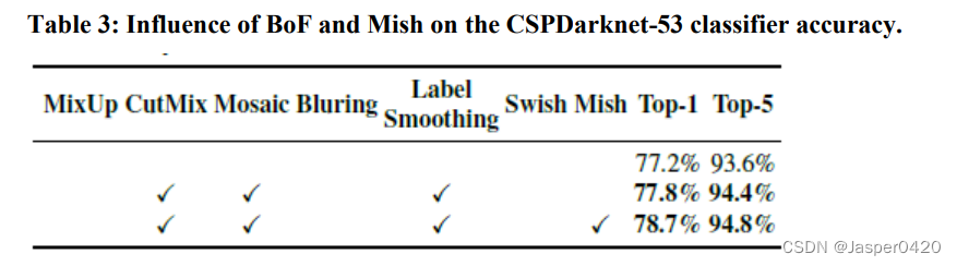
  In our experiments, as illustrated in Table 2, the classifier’s accuracy is improved by introducing the features such as: CutMix and Mosaic data augmentation, Class label smoothing, and Mish activation. As a result, our BoF-backbone (Bag of Freebies) for classifier training includes the following: CutMix and Mosaic data augmentation and Class label smoothing. In addition we use Mish activation as a complementary option, as shown in Table 2 and Table 3.
   As shown in the table 2 Shown , Our experiment introduces the following techniques to improve the accuracy , Such as CutMix And mosaic data enhancement 、 Category label smoothing and Mish Activation function . therefore , Our classifier is trained BoF-backbone (Bag of Freebies) Include CutMix and Mosaic Data to enhance 、 Category label smoothing. besides , As shown in the table 2 And table 3 As shown in, we also use Mish Activate function as complementary option .

4.3 Influence of different features on Detector training The influence of different skills on testing training

  Further study concerns the influence of different Bag-of-Freebies (BoF-detector) on the detector training accuracy, as shown in Table 4. We significantly expand the BoF list through studying different features that increase the detector accuracy without affecting FPS:  S: Eliminate grid sensitivity the equation bx=σ(tx)+cx, by=σ(ty)+cy, where cx and cy are always whole numbers, is used in YOLOv3 for evaluating the object coordinates, therefore, extremely high tx absolute values are required for the bx value approaching the cx or cx+1 values. We solve this problem through multiplying the sigmoid by a factor exceeding 1.0, so eliminating the effect of grid on which the object is undetectable.  M: Mosaic data augmentation – using the 4-image mosaic during training instead of single image  IT: IoU threshold – using multiple anchors for a single ground truth IoU (truth, anchor) > IoU threshold  GA: Genetic algorithms – using genetic algorithms for selecting the optimal hyperparameters during network training on the first 10% of time periods  LS: Class label smoothing – using class label smoothing for sigmoid activation  CBN: CmBN – using Cross mini-Batch Normalization for collecting statistics inside the entire batch, instead of collecting statistics inside a single mini-batch  CA: Cosine annealing scheduler – altering the learning rate during sinusoid training  DM: Dynamic mini-batch size – automatic increase of mini-batch size during small resolution training by using Random training shapes  OA: Optimized Anchors – using the optimized anchors for training with the 512×512 network resolution  GIoU, CIoU, DIoU, MSE – using different loss algorithms for bounded box regression.
   As shown in the table 4 Shown , In depth study of different Bag-of-Freebies (BoF-detector) Under inspection The influence of the tester training . We do not affect... Through research FPS Which can improve the accuracy at the same time skill , Significantly expanded BOF The contents of the list , As follows ：

• S： Eliminates lattice sensitivity , stay YOLOv3 Through the equation bx=σ(tx)+cx, by=σ(ty)+cy Calculate object coordinates , among cx and cy Is always an integer , therefore , When bx It's close to cx or cx+1 It takes a lot of tx The absolute value . We go through take sigmoid Multiply by more than 1.0 To solve this problem , So as to eliminate Have detected the impact of the target grid .
• M： Mosaic data enhancement —— Use during training 4 Mosaic results of images Not a single image
• IT：IoU threshold —— Use multiple... For a truth bounding box anchor,Iou （ Truth value ,anchor）>IoU threshold
• GA： Genetic algorithm (ga) —— At the beginning of network training 10% Using genetic algorithms within a period of time Method to select the optimal hyperparameters
• LS： Category label smoothing—— Yes sigmoid The activation function result uses the class Don't label smoothing
• CBN：CmBN—— Use Cross mini-Batch Normalization Throughout Collect statistical data in small batches , Not in a single mini Collect statistics in small batches data
• CA：Cosine annealing scheduler—— Change the learning rate in sine training  DM：Dynamic mini-batch size—— When using random training shapes , For small resolution input, it is automatically increased mini-batch Size
• OA： optimization Anchors—— Use optimization anchor Yes 512×512 Net of Network resolution for training
• GIoU、CIoU、DIoU、MSE—— Bounding box uses different loss algorithms
  
    Further study concerns the influence of different Bagof-Specials (BoS-detector) on the detector training accuracy, including PAN, RFB, SAM, Gaussian YOLO (G), and ASFF, as shown in Table 5. In our experiments, the detector gets best performance when using SPP, PAN, and SAM.
     As shown in the table 5 Shown , Further research involves different Bag-of-Specials(BoSdetector) The influence on the training accuracy of detector , Include PAN、RFB、SAM、Gaussian YOLO(G) and ASFF. In our experiment , When using SPP、PAN and SAM when , The detector achieves the best performance .
  

4.4 Influence of different backbones and pre-trained weightings on Detector training Different backbone And the influence of pre training weight on detector training

  Further on we study the influence of different backbone models on the detector accuracy, as shown in Table 6. We notice that the model characterized with the best classification accuracy is not always the best in terms of the detector accuracy.

   As shown in the table 6 Shown , We further study different backbone Influence on detector accuracy . We note that model architectures with the best classification accuracy do not always have the best check the accuracy .

  First, although classification accuracy of CSPResNeXt50 models trained with different features is higher compared to CSPDarknet53 models, the CSPDarknet53 model shows higher accuracy in terms of object detection.
   First , Although using different features CSPResNeXt50 The classification accuracy of the model is high On CSPDarknet53 Model , however CSPDarknet53 The model is on the target detection side Higher accuracy .
  Second, using BoF and Mish for the CSPResNeXt50 classifier training increases its classification accuracy, but further application of these pre-trained weightings for detector training reduces the detector accuracy. However, using BoF and Mish for the CSPDarknet53 classifier training increases the accuracy of both the classifier and the detector which uses this classifier pre-trained weightings. The net result is that backbone CSPDarknet53 is more suitable for the detector than for CSPResNeXt50.
   secondly ,CSPResNeXt50 The training of classifiers uses BoF and Mish After that, it was improved Its classification accuracy , However, applying these pre trained weights to the detector training reduces The accuracy of the detector . However ,CSPDarknet53 The classifier is trained using BoF and Mish Both improve the accuracy of the classifier and detector , The detector uses the weight of classifier pre training . The end result is , CSPDarknet53 Than CSPResNeXt50 More suitable for detector Of backbone.
  We observe that the CSPDarknet53 model demonstrates a greater ability to increase the detector accuracy owing to various improvements.
   We observed that ,CSPDarknet53 The model shows greater performance due to various improvements Force to improve the accuracy of the detector .

4.5 Influence of different mini-batch size on Detector training Different mini-batch size Impact on detector training

  Finally, we analyze the results obtained with models trained with different mini-batch sizes, and the results are shown in Table 7. From the results shown in Table 7, we found that after adding BoF and BoS training strategies, the mini-batch size has almost no effect on the detector’s performance. This result shows that after the introduction of BoF and BoS, it is no longer necessary to use expensive GPUs for training. In other words, anyone can use only a conventional GPU to train an excellent detector.
   Last , We analyzed the model through different mini-batch The results of size training , The result chart 7 Shown . From the table 7 From the results shown in , We found that when training, we added BoF and BoS after mini-batch Size has almost no effect on detector performance . This result indicate , introduce BoF and BoS There will be no need to use expensive GPU To train . let me put it another way , Anyone can use only one traditional GPU To train a good detector .

5. Results result

  Comparison of the results obtained with other state-of-the-art object detectors are shown in Figure 8. Our YOLOv4 are located on the Pareto optimality curve and are superior to the fastest and most accurate detectors in terms of both speed and accuracy.
   Pictured 8 The comparison results between our model and other state-of-the-art detectors are shown . I Their YOLOv4 On the Pareto optimal curve , And in terms of speed and accuracy, it is superior to The fastest and most accurate detector .

  Since different methods use GPUs of different architectures for inference time verification, we operate YOLOv4 on commonly adopted GPUs of Maxwell, Pascal, and Volta architectures, and compare them with other state-of-the-art methods. Table 8 lists the frame rate comparison results of using Maxwell GPU, and it can be GTX Titan X (Maxwell) or Tesla M40 GPU. Table 9 lists the frame rate comparison results of using Pascal GPU, and it can be Titan X (Pascal), Titan Xp, GTX 1080 Ti, or Tesla P100 GPU. As for Table 10, it lists the frame rate comparison results of using Volta GPU, and it can be Titan Volta or Tesla V100 GPU.
   Because different methods use different architectures in reasoning time verification GPU, We let YOLOv4 Running on the Maxwell、Pascal and Volta Such as the commonly used GPU On , And compared with other latest technologies . surface 8 Lists the use of Maxwell GPU Time frame rate comparison results , The specific model can be GTX Titan X (Maxwell) or Tesla M40 GPU）. surface 9 Lists the use of Pascal GPU Time frame rate comparison results , The specific model can be Titan X（Pascal）、Titan Xp、GTX 1080 Ti or Tesla P100 GPU. surface 10 List the uses Volta GPU Time frame rate comparison results , Specific model It can be Titan Volta or Tesla V100 GPU.

6. Conclusions Conclusion

  We offer a state-of-the-art detector which is faster (FPS) and more accurate (MS COCO AP 50…95 and AP 50 ) than all available alternative detectors. The detector described can be trained and used on a conventional GPU with 8-16GB-VRAM this makes its broad use possible. The original concept of one-stage anchor-based detectors has proven its viability. We have verified a large number of features, and selected for use such of them for improving the accuracy of both the classifier and the detector. These features can be used as best-practice for future studies and developments.
   We provide a state-of-the-art detector , Compared to all other available 、 Substitutable The detector is faster （FPS）、 More accurate （MS COCO AP50…95 and AP50）. The detector can be used in 8-16GB-VRAM Tradition GPU Train and use , This makes It can be widely used . Based on one stage anchor The original concept of the detector has been Proved to be feasible . We have validated a number of methods , And choose to use some of these methods To improve the accuracy of classifiers and detectors . These methods can be used for future research and development Best practices .