Compare kernelshap and treeshap based on speed, complexity and other factors

KernelSHAP and TreeSHAP Are used for approximation Shapley value .TreeSHAP It's very fast , But it can only be used in tree based algorithms , Such as random forest and xgboost. and KernelSHAP It has nothing to do with the model . This means that it can be used with any machine learning algorithm . We will compare these two approximation methods .

The experiment in this paper , Will show TreeSHAP How fast is it actually . In addition, we also explore how the parameters of tree algorithm affect the time complexity , These include the number of trees 、 Depth and number of features . In the use of TreeSHAP When exploring data , This knowledge is very useful . Finally, we will discuss other factors ( Such as feature dependency ) Some effects of .

This article assumes that you know SHAP, You can refer to other articles published before .

Time per sample

For the first experiment , Let's look at these methods of calculation SHAP How much time does it take . We won't go into detail about the code used , Because the complete code will be provided at the end of this article GitHub Address . Start with simulated regression data . There are 10000 Samples 、10 Characteristics and 1 Continuous target variables . Use the data , We trained a random forest , The model has 100 tree , Maximum depth is 4.

Now you can use this model to calculate SHAP value . Use at the same time KernelSHAP and TreeSHAP Method , Calculate for each method 10、100、1000、2000、5000 and 10000 individual SHAP value . Record the time taken for each value calculation , And I repeat this process 3 Time , Then take the average value as the final time .

You can see it in the picture 1 See results in .TreeSHAP Obviously faster . about 10,000 individual SHAP value , This method is time-consuming 1.44 second . by comparison ,KernelSHAP Time consuming 13 branch 40.56 second . This is a 570 Times of time . Of course, the speed of these calculations will depend on the equipment , But the difference won't be too big .

[ Failed to transfer the external chain picture , The origin station may have anti-theft chain mechanism , It is suggested to save the pictures and upload them directly (img-Jgv4Bvan-1658543917174)(http://images.overfit.cn/upload/20220723/c34a942dca1e4a3e910c9b1d2d465949.png)]

above TreeSHAP The line looks flat . This is because KernelSHAP It's too much . Below 2 in , We draw alone TreeSHAP . It can be seen that it also increases linearly with the increase of observation times . This tells us each SHAP Values need similar time to calculate . We will discuss the reasons in the next section .

Time complexity

The time complexity of the two methods is as follows . This is also the calculation feature of tree algorithm SHAP The complexity of value .T Is the number of individual trees .L Is the maximum number of leaves per tree .D Is the maximum depth of each tree .M Is the maximum number of features in each tree . For these methods , These parameters will affect the approximation time in different ways .

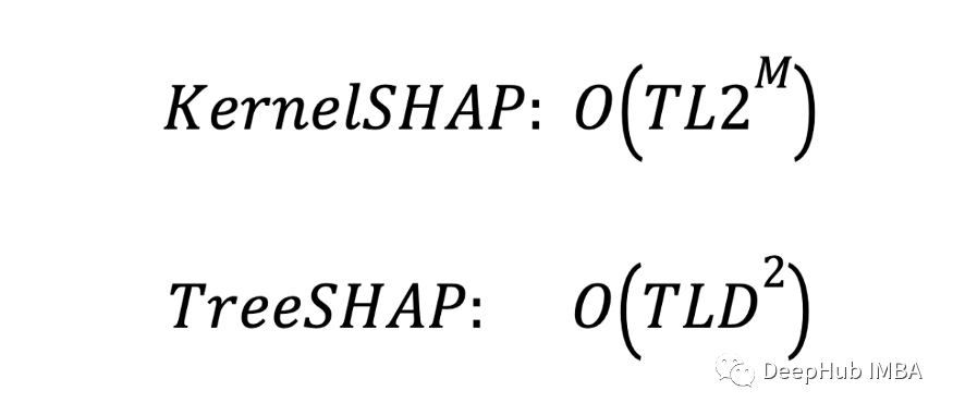
TreeSHAP The complexity of is only affected by depth (D) Influence . and KernelSHAP Affected by the number of features (M) Influence . The difference is KernelSHAP Complexity is exponential w.r.t M and TreeSHAP It's twice w.r.t D. Because the depth of the tree （D=4） Specific characteristics （M = 10） Much smaller , therefore KernelSHAP It's going to be a lot slower .

This is every SHAP Time complexity of value , Generally, each value requires similar time to calculate , So we see that there is a linear relationship between time and the number of observations . Now we will discuss time and other parameters T、L、D and M The relationship between . Then we will discuss the significance of the results to model validation and data exploration .

The number of trees (T)

For both methods , Complexity is the number of trees (T) Linearity of w.r.t.. To verify that this parameter affects the approximation time in a similar way . We train different models by increasing the number of trees , Use each model to calculate 100 individual SHAP value .

You can see it in the picture 3 See results in . For both methods , Time increases linearly with the number of trees . This is what we expect when we look at the time complexity . This tells us , By limiting the number of trees , We can reduce the calculation SHAP The value of the time .

Number of features (M)

Only KernelSHAP Affected by the number of features (M) Influence , This time we train the model on different number of features . Other parameters (T、L、D) remain unchanged . Below 4 in , You can see that with m An increase in ,KernelSHAP The time increases exponentially . by comparison ,TreeSHAP The time is less affected .

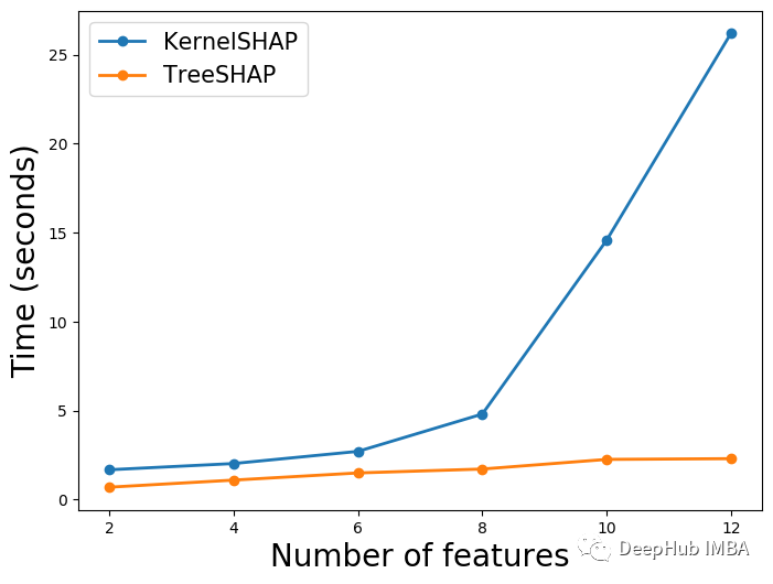
TreeSHAP The time is gradually increasing （ Although it's not obvious ）, Because we see complexity and m irrelevant . This is how to calculate a single feature SHAP The complexity of value . With M An increase in , We need to calculate more for each observation SHAP value , So this increase should be reasonable .

Depth of tree (D)

Last , We change the depth of the tree . We set the depth of each tree in the forest to the maximum depth . Below 5 in , You can see that when we increase the depth, we use TreeSHAP The time has greatly increased . In some cases ,TreeSHAP The calculation cost is even higher than KernelSHAP high . because TreeSHAP Complexity is D Function time , There is no doubt about this .

Why? KernelSHAP Time will also increase ？ It's because of the characteristics (M) Heye (L) The number of varies according to the depth of the tree . As the depth increases , There will be more divisions , So we will have more leaves . More forks also mean that trees can use more features . It can be seen in the figure below 6 See this in . ad locum , We calculated the characteristics of all trees in the forest and the average number of leaves .

Suggestions for model validation and data exploration

By changing the depth , We see in some cases TreeSHAP The calculation cost is higher . But these things are unlikely to happen . Only when the depth of our tree is 20 This happens when . It is not common to use such a deep tree , Because we usually have deeper than the tree (D) More features (M).

In the use of SHAP When validating the tree model ,TreeSHAP Usually a better choice . We can calculate faster SHAP value . Especially when you need to compare multiple models . For model validation , We have parameters T、L、D and M There's not much choice . This is because we only want to verify the model with the best performance .

For data exploration , Tree algorithm can be used to find important nonlinear relationships and interactions . Our model only needs to be good enough to capture potential trends in the data . So by reducing the number of trees (T) And depth (D) To use TreeSHAP Speed up the process . And many model features can be explored without significantly improving the execution time （M）.

Some precautions

When choosing a method , Time complexity is an important factor . Before making a choice , Other differences may need to be considered . These include KernelSHAP It has nothing to do with the model , These methods are affected by feature dependence , And only TreeSHAP It can be used to calculate the interaction effect .

The model is unknowable

We mentioned at the beginning TreeSHAP The biggest limitation of is that it is not model independent . If you use a non tree based algorithm , Will not be able to use it . For example, neural networks also have their own approximation methods . This is what we need to use DeepSHAP. however KernelSHAP Is the only method that can be used with all algorithms .

Feature dependence

Feature dependency may distort KernelSHAP Approximation made . The algorithm estimates by randomly sampling eigenvalues SHAP value . If when features are related , In the use of SHAP When the value of , You may overemphasize unlikely observations .

and TreeSHAP No problem . But because of feature dependency , The algorithm has other problems . That is, features that have no effect on prediction can obtain non-zero SHAP value . When this feature is related to another feature that affects prediction , That's what happens . In this case, the wrong conclusion will be drawn ： That is, a feature contributes to the prediction .

Analyze interactions

SHAP The interaction value is SHAP Extension of value . They decompose the contribution of features into their main and interactive effects . For a given feature , Interaction is all the joint contributions of it and other features . When highlighting and visualizing interactions in data , These may be useful . If you need this content , We can introduce it in a separate article .

If you want to use SHAP Interaction value , Must be used TreeSHAP. This is because it is the only approximate method to realize the interaction value . This is related to SHAP The complexity of interaction values . Estimate these KernelSHAP need Longer time .

summary

Should be used whenever possible TreeSHAP. It's faster , And be able to analyze interactions . For data exploration . If you are using other types of model algorithms , Then you will have to insist on using KernelSHAP., Because it is still a faster approximation method than other methods such as Monte Carlo sampling .

The complete code of this article ：
https://avoid.overfit.cn/post/74f491a38a874b5e8dd9d17d9da4bfbb

author ：Conor O’Sullivan