[don't bother to strengthen learning] video notes (IV) 2. Dqn realizes maze walking

The first 11 section DQN Realize the maze ——《 Strengthen learning notes 》

---

In the previous section, we have introduced in detail DQN The two sharp weapons of ：REPLAY BUFFER（ Empirical playback mechanism ） and frozen Q-target（ Target network , Two networks are used to estimate the truth Q Value network ）, Here is given DQN The pseudo code , Convenient for later programming .

---

11.1 Main circulation

DQN The pseudocode is as follows :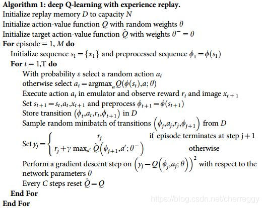

The main code of the main loop is the above update process , Other things like DQN Class and other codes are supplemented later . The main loop should pay attention to , Here are two networks and REPLAY BUFFER Usefulness , Is to cut off the correlation between Markov sequence elements .
For the preparation of the network 、 The main function of network parameter update is not considered , Intermediate storage to REPLAY BUFFER The following content belongs to learning Q Content of the network , All in DQN Class learn Function .
Here we also add the drawing function of neural network error dotted line , If you can , You can also modify the code , Output all of the two networks LOSS Changes .

from maze_env import Maze
from DQN import DeepQNetwork


def run_maze():
    step = 0    #  Record the steps , It is used to prompt the time of learning 
    for episode in range(300):
        #  Initialization environment 
        observation = env.reset()
        while True:
            env.render()  #  Render a frame of environment 
            action = RL.choose_action(observation)  # DQN According to the current state s Choose behavior a
            observation_, reward, done = env.step(action)  #  Interact with the environment , Get the next status s'、 Reward R And whether it reaches the final state 
            RL.store_transition(observation, action, reward, observation_)  #  Store the current sampling sequence in RF in （s, a, R, s'）

            # 200 Start learning after step , every other 5 Step by step , to update Q Network parameters （ The first network ）
            if (step > 200) and (step % 5 == 0):
                RL.learn()

            observation = observation_  #  Move to the next state 
            if done:  #  If terminated ,  Just jump out of the loop 
                break
            step += 1   #  Total steps  + 1

    #  Game over 
    print('game over')
    env.destroy()


if __name__ == "__main__":
    env = Maze()  #  Create an environment 
    RL = DeepQNetwork(env.n_actions, env.n_features,
                      learning_rate=0.01,
                      reward_decay=0.9,
                      e_greedy=0.9,
                      replace_target_iter=200,  #  Every time  200  Step change once  target_net  Parameters of 
                      memory_size=2000, #  Memory limit 
                      # output_graph=True #  Whether the output  tensorboard  file 
                      )
    env.after(100, run_maze)
    env.mainloop()
    RL.plot_cost()  #  Error curve of neural network 

---

11.2 DeepQNetwork class

DQN And Q Learning and SARSA There's a big difference , The code of the main class contains Parameter initialization 、 Creating networks 、 Store memory 、 Choose action 、 Study and Draw the learning curve These modules .

Parameter initialization

The specific parameter meanings are in the code comments .

import tensorflow as tf
import numpy as np


class DeepQNetwork:
    def __init__(
            self,
            n_actions,
            n_features,
            learning_rate=0.01,
            reward_decay=0.9,
            e_greedy=0.9,
            replace_target_iter=300,
            memory_size=500,
            batch_size=48,
            e_greedy_increment=None,
            output_graph=False,
    ):
        self.n_actions = n_actions  #  Action space , There are several movements 
        self.n_features = n_features  #  The dimensions of characteristics , For example, the maze is the position in the maze (length, height), Image words may be (m*n) Size picture 
        self.lr = learning_rate  #  Learning rate , Parameter update efficiency 
        self.gamma = reward_decay  #  Reward decay factor 
        self.epsilon_max = e_greedy  # epsilon-greedy Parameters of , The larger the number, the smaller the randomness 
        self.replace_target_iter = replace_target_iter  #  Update the target network every few steps （ The second network ）
        self.memory_size = memory_size  #  Memory limit 
        self.batch_size = batch_size  #  Every update from buffer The number of memories taken out 
        self.epsilon_increment = e_greedy_increment  # epsilon The value of increases with time , That is, the randomness decreases , Explore mode parameters 
        self.epsilon = 0 if e_greedy_increment is not None else self.epsilon_max  #  Whether to turn on discovery mode ,
        #  And gradually reduce the number of explorations ,epsilon by 0 The proof is completely random at first 

        self.learn_step_counter = 0  #  Record the number of learning steps , To update the target network parameters 

        #  Initialize all  0  memory  [s, a, r, s_]
        self.memory = np.zeros((self.memory_size, n_features * 2 + 2))  # *2 It means observed value （ state ） It's two-dimensional （ coordinate ）

        self._build_net()  #  establish Q Network and target network 

        #  Replace  target net  Parameters of 
        t_params = tf.get_collection('target_net_params')  #  Extract the parameters of the target network 
        e_params = tf.get_collection('eval_net_params')  #  extract Q Network parameters 
        self.replace_target_op = [tf.assign(t, e) for t, e in zip(t_params, e_params)]  #  Update target network parameters 

        self.sess = tf.Session()

        #  Output log file 
        if output_graph:
            # $ tensorboard --logdir=logs  Input mode of command line , see tensor board command 
            tf.summary.FileWriter("logs/", self.sess.graph)

        self.sess.run(tf.global_variables_initializer())  #  Initialize global parameters 
        self.cost_his = []  #  Record all loss,  For final drawing 

Notice the top Q The Internet It refers to sampling and from buffer Generated when taking out memory Q Value network （ abbreviation Network one ）, Target network It refers to the estimation of truth in learning update Q value , Networks that update slower than the former （ abbreviation Network II ）, Two networks The structure is exactly the same , But the parameter update step of the second network is larger （ Assign network one parameter to network two at regular intervals ）.

Creating networks

There are some difficulties in the code of network creation , Need to use tensor flow, Here is only a simple description and code , Other parts will not be explained in detail . The specific structure of the network can be found in tensor board View in ,tensorboard Usage method ：Tensorboard The use of,
Specifically about the network structure and Tensorboard For visual results, please look down the article .

    def _build_net(self):
        # ------------------  establish Q The Internet  ------------------
        self.s = tf.placeholder(tf.float32, [None, self.n_features], name='s')  #  Input status s
        self.q_target = tf.placeholder(tf.float32, [None, self.n_actions], name='Q_target')  #  Used to store the target Q value 
        with tf.variable_scope('eval_net'):
            # c_names： A collection of storage parameters 
            c_names, n_l1, w_initializer, b_initializer = \
                ['eval_net_params', tf.GraphKeys.GLOBAL_VARIABLES], 10, \
                tf.random_normal_initializer(0., 0.3), tf.constant_initializer(0.1)  #  Parameter initializer 

            #  first floor , Linear polynomial , Parameters are used when copying to the target network 
            with tf.variable_scope('l1'):
                w1 = tf.get_variable('w1', [self.n_features, n_l1], initializer=w_initializer, collections=c_names)
                b1 = tf.get_variable('b1', [1, n_l1], initializer=b_initializer, collections=c_names)
                l1 = tf.nn.relu(tf.matmul(self.s, w1) + b1)

            #  The second floor 
            with tf.variable_scope('l2'):
                w2 = tf.get_variable('w2', [n_l1, self.n_actions], initializer=w_initializer, collections=c_names)
                b2 = tf.get_variable('b2', [1, self.n_actions], initializer=b_initializer, collections=c_names)
                self.q_eval = tf.matmul(l1, w2) + b2

        with tf.variable_scope('loss'):
            self.loss = tf.reduce_mean(tf.squared_difference(self.q_target, self.q_eval))
        with tf.variable_scope('train'):
            self._train_op = tf.train.RMSPropOptimizer(self.lr).minimize(self.loss)

        # ------------------  Build the target network , and Q The network is exactly the same ------------------
        self.s_ = tf.placeholder(tf.float32, [None, self.n_features], name='s_')  #  Input 
        with tf.variable_scope('target_net'):
            c_names = ['target_net_params', tf.GraphKeys.GLOBAL_VARIABLES]

            #  first floor 
            with tf.variable_scope('l1'):
                w1 = tf.get_variable('w1', [self.n_features, n_l1], initializer=w_initializer, collections=c_names)
                b1 = tf.get_variable('b1', [1, n_l1], initializer=b_initializer, collections=c_names)
                l1 = tf.nn.relu(tf.matmul(self.s_, w1) + b1)

            #  The second floor 
            with tf.variable_scope('l2'):
                w2 = tf.get_variable('w2', [n_l1, self.n_actions], initializer=w_initializer, collections=c_names)
                b2 = tf.get_variable('b2', [1, self.n_actions], initializer=b_initializer, collections=c_names)
                self.q_next = tf.matmul(l1, w2) + b2

Store memory

here REPLAY BUFFER The size of is fixed , The variables above memory_size Namely buffer Size , The index loop points to each row , The new memory will cover the old one .

    def store_transition(self, s, a, r, s_):
        if not hasattr(self, 'memory_counter'):  #  Check whether the variable exists 
            self.memory_counter = 0  #  Record the total number of memories 

        #  Record a  [s, a, r, s_]  Record 
        transition = np.hstack((s, [a, r], s_))  #  Become a horizontal vector 

        #  total  memory  The size is fixed ,  If it exceeds the total size ,  used  memory  By the new  memory  Replace 
        index = self.memory_counter % self.memory_size  #  Similar to a circular array , Take the remainder and place it circularly , Cover the previous content 
        self.memory[index, :] = transition  #  Place memory 
        self.memory_counter += 1  #  Number of memory strips +1

Action selection

First enter Q The network gets all the action Q value , according to $ϵ$-Greedy Select action index output .

    def choose_action(self, observation):
        #  stay observation Add a dimension before (1, size_of_observation), For convenience tensor flow Handle 
        observation = observation[np.newaxis, :]
        if np.random.uniform() < self.epsilon:  # epsilon Probability of greedy choice 
            actions_value = self.sess.run(self.q_eval, feed_dict={
    self.s: observation})  #  Input status , Output the corresponding Q value 
            action = np.argmax(actions_value)  #  Choose the largest action 
        else:
            action = np.random.randint(0, self.n_actions)   #  Random selection 
        return action

Study

Here's the key code , Corresponding to the pseudo code flow above .

• First, through $ϵ$-Greedy Get the action a, Interaction with the environment is rewarded R And the next state s’. Put this experience sequence $(s,a,R,s^{\prime },end?)$ Put in buffer in , among $end?$ Indicates whether it is the final state .
• When updating the network , from buffer Take out a batch of experience sequence , First put it $s^{\prime }$ Input to Q The network gets the predicted action Q Value corresponds to the maximum action , That is... In the code $ma{x}_{a^{\prime }}\hat{Q}({\varphi }_{j+1},a^{\prime };{\theta }^{-})$. Multiplied by $\gamma$（ Attenuation coefficient ） add r（ Reward ） Estimated True value .
• Then put the corresponding state $s$ And the action $a$ Input to Q Get in the network Estimated value .
• True value and Estimated value Do a bad job and get LOSS, Use LOSS Update the gradient descent method Q Network parameters
• Update every certain step Target network

    def learn(self):
        #  Reaching a certain number of steps will Q The parameters of the network are copied to the target network 
        if self.learn_step_counter % self.replace_target_iter == 0:
            self.sess.run(self.replace_target_op)
            print('\ntarget_params_replaced\n')

        #  from  buffer(memory) Randomly selected from  batch_size  Memory of size 
        if self.memory_counter > self.memory_size:  #  exceed buffer The size selection range is buffer Size 
            sample_index = np.random.choice(self.memory_size, size=self.batch_size)  #  Otherwise, it is the size of the number of existing memory , Avoid extracting empty memories into 
        else:
            sample_index = np.random.choice(self.memory_counter, size=self.batch_size)
        batch_memory = self.memory[sample_index, :]  #  Get a batch of memory to update the network 

        #  obtain  q_next ( The target network generates )  and  q_eval(Q Network generation )
        q_next, q_eval = self.sess.run(
            [self.q_next, self.q_eval],
            feed_dict={
    
                self.s_: batch_memory[:, -self.n_features:],
                self.s: batch_memory[:, :self.n_features]
            })

        #  The following steps are very important . q_next, q_eval  Contains all the  action  Value ,
        #  And all we need is what we have chosen  action  Value ,  Others don't need .
        #  So we're going to other  action  All values become  0,  Will be used  action  Error value   Reverse pass back ,  As update credentials .
        #  This is what we finally want to achieve ,  such as  q_target - q_eval = [1, 0, 0] - [-1, 0, 0] = [2, 0, 0]
        # q_eval = [-1, 0, 0]  It means that I have chosen... In this memory  action 0,  and  action 0  It brings  Q(s, a0) = -1,  So the others  Q(s, a1) = Q(s, a2) = 0.
        # q_target = [1, 0, 0]  It means... In this memory  r+gamma*maxQ(s_) = 1,  And no matter in  s_  Which one did we take last time  action,
        #  We all need to correspond to  q_eval  Medium  action  Location ,  So I will  1  On the  action 0  The location of .

        #  The following is also to achieve the above purpose ,  But in order to make the program operate more ,  The process of achieving the goal is a little different .
        #  Yes, it will  q_eval  Assign all values to  q_target,  At this time  q_target-q_eval  All for  0,
        #  however   Let's go back to  batch_memory  In the middle of  action  This  column  Here it is  q_target  The corresponding of  memory-action  Position to modify the assignment .
        #  Make the new assignment  reward + gamma * maxQ(s_),  such  q_target-q_eval  Can become what we need .
        #  There is another example below .

        q_target = q_eval.copy()
        batch_index = np.arange(self.batch_size, dtype=np.int32)
        eval_act_index = batch_memory[:, self.n_features].astype(int)
        reward = batch_memory[:, self.n_features + 1]

        q_target[batch_index, eval_act_index] = reward + self.gamma * np.max(q_next, axis=1)

        """  If in this  batch  in ,  We have 2 An extracted memory ,  According to each memory, we can produce 3 individual  action  Value : q_eval = [[1, 2, 3], [4, 5, 6]] q_target = q_eval = [[1, 2, 3], [4, 5, 6]]  And then according to  memory  The specific  action  Position to modify  q_target  Corresponding  action  Value on :  For example :  memory  0  Of  q_target  The calculated value is  -1,  And I used  action 0;  memory  1  Of  q_target  The calculated value is  -2,  And I used  action 2: q_target = [[-1, 2, 3], [4, 5, -2]]  therefore  (q_target - q_eval)  It becomes : [[(-1)-(1), 0, 0], [0, 0, (-2)-(6)]]  Finally, we put this  (q_target - q_eval)  As an error ,  Back propagation neural network .  All for  0  Of  action  The value was not chosen at that time  action,  There was a choice before  action  There is nothing to do 0 Value .  We only reverse the previously selected  action  Value , """

        #  Training  eval_net
        _, self.cost = self.sess.run([self._train_op, self.loss],
                                     feed_dict={
    self.s: batch_memory[:, :self.n_features],
                                                self.q_target: q_target})
        self.cost_his.append(self.cost) #  Record  cost  error 

        #  Gradually increase  epsilon,  Reduce the randomness of behavior 
        self.epsilon = self.epsilon + self.epsilon_increment if self.epsilon < self.epsilon_max else self.epsilon_max
        self.learn_step_counter += 1

Draw the learning curve

    def plot_cost(self):  #  Visualize learning results 
        import matplotlib.pyplot as plt  #  Yes  pyplot Visualization Library 
        plt.plot(np.arange(len(self.cost_his)), self.cost_his)
        plt.ylabel('Cost')
        plt.xlabel('training steps')
        plt.show()

---

11.3 The operation effect is similar to tensorboard

have NVIDIA The graphics card can be used to run code , It's going to be a lot faster , Please find Baidu by yourself for specific methods . The following is the running interface effect ：

If you are using PYCHARM, Then you can click on the console below terminal, Bring up the terminal , Input tensorboard --logdir logs, Show the following ：

(base) F:\ Reinforcement learning \DQN>tensorboard --logdir logs
TensorBoard 1.14.0 at http:// Computer information number （ It's not convenient to give ）:6006/ (Press CTRL+C to quit)

Open any browser , Address field input localhost:6006, Visit to see tensorboard Network structure diagram displayed on the interface ：
LOSS Change the following ：

---

11.4 About dual networks and Replay Buffer The understanding of the

From the above network structure diagram, we can clearly see the following points ：

1. Q The Internet （eval_net） Input status s, Target network (target_net) Input status s’, Both outputs get LOSS
2. Q The network will pass its parameter values to the target network
3. Only Q The network is updating parameters

and Replay Buffer The existence of , It was also introduced before that the purpose is Weaken the correlation between time series , I drew a picture to show Replay Buffer The role and process of ：

In fact, the fixed size storage space in the code can be used as Circular queue Use , The effect is to let the new memory cover the old memory . So how do batch memories update at the same time ？ How does the dimension change ？
Here I also draw an image to show the dimensional changes in the process （ But the corresponding example in this figure is not a maze , It was written before Atari Examples of games , The input is the image , Of course, the network structure is also different ）：

Of course , There are still many places worth exploring , For example, the structure of the network （ But the network structure is very complex , A wide range ）、batch_size and replay buffer The impact of the size of on the running results , You can try it in code . You can also try other environments , stay OpenAI Gym There are many environments , Please refer to for specific usage ：OpenAI gym Environment library

Last one ：【 Don't bother to strengthen learning 】 Video notes （ Four ）1. What is? DQN？
Next ：【 Don't bother to strengthen learning 】 Video notes （ 5、 ... and ）1. What is the strategic gradient ？