Data analysis of time series (III): decomposition of classical time series

I have completed the previous two blogs , Readers who haven't read it yet please read it first ：

1. Data analysis of time series ( One ): The main ingredients

2. Data analysis of time series ( Two ): Calculation of data trend

5、 ... and . Time series decomposition

        It has been introduced before that the seasonal characteristics of time series data can be divided into additive seasonality and multiplicative seasonality , Therefore, there are two methods to decompose time series data: additive decomposition and multiplicative decomposition . The following methods are manual and automatic ( call statsmodes.seasonal_decompose) To achieve decomposition , The reason for using manual method is to let readers thoroughly understand the built-in logic of time series decomposition .

5.1 Judgment of seasonal cycle

The data of time series often show the law of periodic change , This cyclical change law is often brought about by seasonal factors , If the time granularity of your time series data is time ( Such as hours ), Then its seasonal cycle may be 24, If the granularity of time is days , The seasonal cycle may be 7, If the time granularity is month , The seasonal cycle may be 12, If the time granularity is quarterly , Then its seasonal cycle may be 4. Now let's look at the trend chart of the data set of the number of international airlines .

df=pd.read_csv("airline_Passengers.csv")
df['Period']=pd.to_datetime(df['Period'])
df.plot(x='Period',y='#Passengers',title="Airline passengers",figsize=(10,6));
xcoords = ['1950-01', '1951-01', '1952-01', '1953-01', '1954-01',
           '1955-01', '1956-01', '1957-01', '1958-01', '1959-01-01','1960-01']
for xc in xcoords:
    plt.axvline(x=xc, color='blue', linestyle='--')

The time range of this data set ranges from 1949-1960 common 12 year , The granularity of time is month , That is, every month 1 Data 12 Year total 144 Monthly data , Because there are 12 Months , Therefore, it is generally believed that the seasonal cycle of this data set is 12, That is, every 12 Monthly data will fluctuate periodically , This can be seen from the variation law of the data within the blue vertical lines in the above figure ( The blue vertical line is at the beginning of each year ), The data in the above figure is every 12 There are periodic fluctuations in months and the annual fluctuation range will gradually increase , This shows the seasonal characteristics of multiplication .

5.2 Additive decomposition ( Manual method )

step 1: Calculate the trend period term

If the seasonal cycle m When it is an odd number, we use the simple moving average method to calculate the trend periodic term , The box m-MA To calculate the trend period term   , If seasonal cycle m For even numbers 2×m-MA To calculate the trend period term , In the above example, the seasonal cycle is 12 Is an even number, so you need to use 2×m-MA To calculate the trend period term .

order=12
df[str(order)+'-MA']=df['#Passengers'].rolling(window=order).mean().shift(-int(order/2))
df['2×12-MA']=df[str(order)+'-MA'].rolling(window=2).mean()

  step 2： Calculate the detrended sequence

We need to remove the impact of trends from the original data set , The box #Passengers Example subtraction 2×12-MA Column gets a new column ：detrended

df['detrended']=df['#Passengers']-df['2×12-MA']
df.plot(x='Period',
        y=['#Passengers','2×12-MA','detrended'],
        ylabel='#Passengers',figsize=(10,6));

step 3： Calculate the seasonal term

The basic idea of calculating the seasonal term is :1. According to the time granularity of the data ( Hours 、 God 、 month 、 season 、 Years etc. ) Calculate average ( For example, if the time granularity of the data is month , Then calculate every month (1-12 month ) Average value in all years ),2. Subtract the detrended value from these averages (detrended) Average value , 3. Expand the number of results .

# Number of records 
num_data=df.shape[0]
# Seasonal cycle 
period=12
#1. Calculate monthly average 
df['month']=df.Period.apply(lambda x:pd.to_datetime(x).month)
month_mean=df.groupby('month').detrended.mean().values
#2. Monthly average minus trend average 
detrended_month_mean=month_mean-df.detrended.mean()
#3. Expand the number of results 
df['seasonal'] = np.tile(detrended_month_mean,num_data //period)[:num_data]
df=df.drop(['month'],axis=1) 

df.plot(x='Period',
        y=['#Passengers','2×12-MA','seasonal'],
        ylabel='#Passengers',figsize=(10,6));

  step 4： Calculated residual error

The calculation of residual error is relatively simple as long as the trend value is removed (detrended) Subtract the seasonal items (seasonal) You can get the residual ：

# Calculated residual error 
df['resid']=df.detrended-df.seasonal
df.plot(x='Period',
        y=['#Passengers','2×12-MA','resid'],
        ylabel='#Passengers',figsize=(10,6));

  Finally, put the trend 、 Season item 、 The residuals are displayed together ：

df['Period'] = pd.to_datetime(df['Period'])
plt.figure(figsize=(10,8))
plt.subplot(4,1,1)
plt.plot(df.Period.values,df['#Passengers'].values)
plt.ylabel('#Passengers');
plt.title('Additive Decomposition');
plt.subplot(4,1,2);
plt.plot(df.Period.values,df['2×12-MA'].values)
plt.ylabel('trend')
plt.subplot(4,1,3);
plt.plot(df.Period.values,df['seasonal'].values)
plt.ylabel('seasonal')
plt.subplot(4,1,4);
plt.scatter(df.Period.values,df['resid'].values)
plt.ylabel('resid');

 

 5.3 Multiplicative decomposition ( Manual method )

step 1: Calculate the trend period term

Same as addition

step 2： Calculate the detrended sequence

Divide the raw data by the trend , The box #Passengers example Divide 2×12-MA Column gets a new column ：detrended

df['detrended']=df['#Passengers']/df['2×12-MA']

step 3： Calculate the seasonal term

The basic idea of calculating the seasonal term is :1. According to the time granularity of the data ( Hours 、 God 、 month 、 season 、 Years etc. ) Calculate average ( For example, if the time granularity of the data is month , Then calculate every month (1-12 month ) Average value in all years ),2. Average these values again Divide Detrend value (detrended) Average value , 3. Expand the number of results .

# Number of records 
num_data=df.shape[0]
# Seasonal cycle 
period=12
#1. Calculate monthly average 
df['month']=df.Period.apply(lambda x:pd.to_datetime(x).month)
month_mean=df.groupby('month').detrended.mean().values
#2. Divide the monthly average by the trend average 
detrended_month_mean=month_mean/df.detrended.mean()
#3. Expand the number of results 
df['seasonal'] = np.tile(detrended_month_mean,num_data //period)[:num_data]
df=df.drop(['month'],axis=1) 

step 4： Calculated residual error

The calculation of residuals is relatively simple, as long as the original data is divided by the trend and seasonal product You can get the residual, that is : data/(trend*seasonal)

df['resid'] =df['#Passengers']/(df['2×12-MA']*df.seasonal)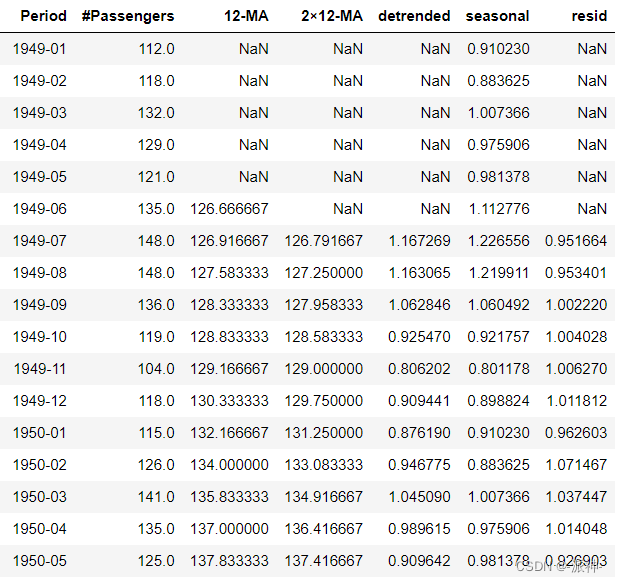

  Finally, put the trend 、 Season item 、 The residuals are displayed together ：

df['Period'] = pd.to_datetime(df['Period'])
plt.figure(figsize=(10,8))
plt.subplot(4,1,1)
plt.plot(df.Period.values,df['#Passengers'].values)
plt.ylabel('#Passengers');
plt.title('Multiplicative decomposition');
plt.subplot(4,1,2);
plt.plot(df.Period.values,df['2×12-MA'].values)
plt.ylabel('trend')
plt.subplot(4,1,3);
plt.plot(df.Period.values,df['seasonal'].values)
plt.ylabel('seasonal')
plt.subplot(4,1,4);
plt.scatter(df.Period.values,df['resid'].values,s=15)
plt.ylabel('resid');

 

 5.3 Use statsmodels Package to automatically decompose time series

Let's use statsmodels Package to decompose time series , We will call statsmodels Of seasonal_decompose Method , And by setting parameters mode="additive(multiplicative)" To perform addition ( Multiplication ) Decomposition operation ：

from statsmodels.tsa.seasonal import STL, seasonal_decompose
plt.rc("figure", figsize=(10, 6))
df=pd.read_csv("airline_Passengers.csv")
df.set_index('Period',inplace=True)
df.index = pd.to_datetime(df.index)
data = df["#Passengers"]
seasonal_decomp = seasonal_decompose(data, model="additive",period=12)
df['trend']=seasonal_decomp.trend
df['seasonal']=seasonal_decomp.seasonal
df['resid']=seasonal_decomp.resid
seasonal_decomp.plot();

  

From the data results in the figure above, we find that the results of automatic addition and decomposition are consistent with those of our manual decomposition .

summary

In this chapter, we learned the basic steps of additive decomposition and multiplicative decomposition of time series data , We calculated the trend step by step by hand 、 Go to the trend item 、 Season item 、 Residual term and other characteristic terms , The purpose of manual decomposition is to enable readers to further understand the calculation logic of each feature item , Finally, we used statsmodels Of seasonal_decompose Method to automatically decompose , The results of manual decomposition and automatic decomposition are compared , And confirm that they are consistent .