Data analysis of time series (II): Calculation of data trend

Four , Decomposition of time series

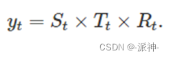
Because seasonal elements are divided into additive seasonality and multiplicative seasonality , Seasonality of addition has nothing to do with time , There is a linear relationship between the seasonality of multiplication and time , Therefore, there are two ways to decompose time series data: additive decomposition and multiplicative decomposition , If time series data show additive seasonal characteristics , Then at any time in the data t The value of can be determined by seasonality , Add the trend and residual to get ：

  In the upper form  y(t) Represents time series data ,S(t) Indicates seasonal items ,T(t) Represents a trend item - Periodic term ,R(t) Represents the residual term .

If the time series data show the seasonal characteristics of multiplication , Then at any time in the data t The value of can be determined by seasonality , Multiply the trend and residual to get ：

 4.1, Trend calculation

We hope that the trend curve of time series data will be as smooth as possible , The first step of the traditional time series decomposition method is to use the moving average method to estimate the trend - Periodic term

4.1.1 Simple moving average

m  The order moving average can be defined as ：

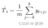
among ,m=2k+1. in other words , Point in time t The trend of is estimated by finding t The value of the moment ±k The average value in a time period . When time is near , Observations are also likely to be close to . thus , The average eliminates some randomness in the data , Thus we can get a smoother trend period , Let's call it alpha “m-MA”, That is to say m Order moving average . Let's take a look at the trend chart of Australia's total exports over the years , Then let's analyze the trend of moving average of different orders .

import pandas as pd

df = pd.read_csv("Australia_economy.csv")
df = df[['Year','Exports']].set_index('Year')
df.plot(xlabel='Year',
        ylabel='% of GDP',
        title='Total Australian exports',
        figsize=(10,6));

Let's look at 5 Step moving average ：

df = pd.read_csv("Australia_economy.csv")
df = df[['Year','Exports']].set_index('Year')
# produce 5 Order moving average 
order1=5
df[str(order1)+'-MA']=df['Exports'].rolling(window=order1).mean().shift(-int((order1-1)/2))
# visualization 
df.plot(xlabel='Year',
        ylabel='% of GDP',
        title='5-MA',
        figsize=(6,5));

We observed that in 5-MA This column is in 1960 and 1961 The value of these two years is empty , This is because m=2k+1, In order to maintain the symmetry of the data , We keep the header and footer of the dataset k Null data , here m be equal to 5 therefore k=2, Therefore, there are both headers and tails of the dataset 2 Null data ( The tail null data is not displayed ).python When realizing the symmetry effect of moving average, we use pandas Of rolling and shift Method , First, through rolling and mean To achieve moving average , And then use shift To achieve data symmetry . Similarly, we can draw 3-MA,5-MA,7-MA,9-MA To compare their direct trend changes ：

From the above figure, we observe that when m As we grow older , The moving average is becoming smoother ,  The order of the moving average determines the trend - The smoothness of the periodic term . In general , The greater the degree, the smoother the curve . The order of simple moving average is often odd （ for example 3,5,7 etc. ）, This ensures symmetry . At order m=2k+1 Moving average , The center observation value and both sides have k Observations can be averaged . But if m It's even , Then it no longer has symmetry .

4.1.2 Even order moving average

When time series data show even order trend changes ( Such as quarter :4, monthly :12), Simple moving average “m-MA” Unable to maintain data symmetry , In order to achieve data symmetry, we need to m-MA Do it again on the basis of 2 Order moving average , This method is called "2×m-MA", Let's take a look at the data of beer production in Australia over the years , This data set records the quarterly beer production in Australia over the years , Because there are 4 Quarterly , So here we want to achieve an even order moving average , The specific steps are to realize an even order (4) The moving average of , Because the result of even order moving average is asymmetric , In order to make the data symmetrical, we need to do it again on the basis of even order moving average 2 The moving average of order is 2×m-MA, Let's first look at the trend chart of this data , Then we will realize 2×m-MA The moving average of ：

df=pd.read_csv('ausbeer2.csv')
df = df[df.date>='1992-01-01']
df.plot(x='date',y='Production',figsize=(10,6),ylabel='Production');

# Realization 4-MA Moving average 
order=4
df[str(order)+'-MA']=df['Production'].rolling(window=order).mean().shift(-int(order/2))
# Realization 2×4-MA" Moving average 
df['2×4-MA']=df['4-MA'].rolling(window=2).mean()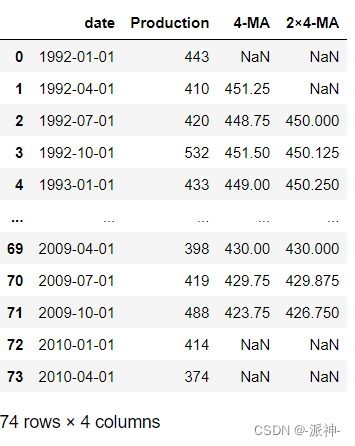

  As can be seen from the results above 4-MA The result is asymmetric ( The head has 1 Null data , The tail has 2 Null data ), and 2×4-MA The result is symmetrical ( Head and tail have 2 Null data ). The last column of data 2×4 -MA The function of is to carry on 4-MA After that 2-MA. The value of the last column is determined by the data of the previous column 2 Obtained after order moving average .4-MA The first two values in the column are ： 451.25=(443+410+420+532)/4 and 448.75=(410+420+532+433)/4. and 2x4-MA The first value of the column is the average of the two ： 450.00=(451.25+448.75)/2. We can  2×4-MA It's written in the form ：

In general , After even order moving average, another even order moving average should be carried out to make it symmetrical . Here we observe  2×4-MA Result ：

Before odd order (m-MA) In the moving average method, the weights of each observation value are equal, and they are 1/m, However, in the even order (2×m-MA) In the moving average method, the weight of the final measured value is  1/(2m), The weights of other observations are 1/m, In the above 2×4-MA For example , The weight of each observation is ：[1/8,1/4,1/4,1/4,1/8] They correspond to 5 An observation . It can be seen that the moving average of even order can be converted into the weighted moving average of odd order, that is 2×m-MA<==>(m+1)-MA. In general , weighting  m-MA Can be written as ：

In the upper form k=(m-1)/2, Its weight is ： [1/(2m), 1/m……1/m, 1/(2m)] And the sum of all weights is 1, And they are symmetrical . 

4.1.3 Why weight

The weighting here refers to a group of observations with unequal weight values , Then why add different weight values to each observation ？ In the above data set of Australian beer production , The time scale of the data is quarter , In a year 4 Quarterly , Therefore, the trend should be obtained by moving average of even order - Periodic term , However 2×4-MA But for continuous 5 The observations are weighted , front 4 Observations are considered to be in the same year 4 Quarterly , The first 5 Observations for the first quarter of the second year , stay 5 The smaller of the first and last weight values is 1/(2m), Other weight values are 1/m, Smaller closing weight value can reduce the fluctuation of data in consecutive years, which can be understood here as preventing large data fluctuation in the first quarter of the second year , Such a small weight value can make the trend curve smoother .

4.2 summary

In this chapter, we learned that time series decomposition methods include additive decomposition and multiplicative decomposition , The trend of data can be calculated by moving average , Moving average can be divided into simple moving average ( Odd order ) And even order moving average , The result of simple moving average is symmetric , The result of even order moving average is asymmetric , For this reason, we need to carry out even order moving average again to make the data symmetrical , Similarly, even order moving average 2×m-MA It can be converted into odd order moving average (m+1)-MA, And the weight is : [1/(2m), 1/m……1/m, 1/(2m)], Among them, the small weight value at the beginning and end is to overcome the impact of data fluctuations in consecutive years on the trend , And make the trend curve smoother .