[machine learning] wuenda's machine learning assignment ex2 logistic regression matlab implementation

Content review

1.1 The hypothesis is that

$$h(x)=g({\theta }^{T}X)$$
$$g(z)=\frac{1}{1+e^{-z}}$$
$h_{\theta }(x)$ The role of is , For a given input variable , Calculate the output variable according to the selected parameter =1 The possibility that $h_{\theta }(x)=P(y=1|x;\theta )$
Hypothesis simplification results in
$$h(x)=\frac{1}{1+e^{-{\theta }^{T}x}}$$

1.2 Determine the boundary

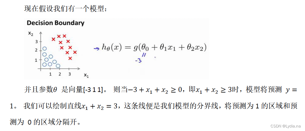
The function that separates the regions is the dividing line of the model .

1.3 Cost function

$$J(\theta )=\frac{1}{m}\sum _{i=1}^m[-y^{(i)}log(h_{\theta }(x^{(i)}))-(1-y^{(i)})log(1-x^{(i)}))]$$
$$\frac{\partial J(\theta )}{\partial {\theta }_j}=\frac{1}{m}\sum _{i=1}^m(h_{\theta }(x^{(i)})-y^{(i)})x^{(i)}$$

1.4 Advanced optimization

Gradient descent can be used to calculate the cost function and the partial derivative of the cost function . However, there are some more advanced algorithms to solve the above two ： The local optimization method is also called conjugate gradient method （BFGS） And finite memory local optimization （LBFGS）. Algorithm advantages ： There is no need to manually select the learning rate in any of these algorithms $\alpha$, It has an intelligent internal loop , It is called linear search , You can automatically try different learning rates .

1.5 Regularization

Add regularization term to solve over fitting problem .
The cost function of regularized linear regression ：
$$J(\theta )=\frac{1}{2m}\sum _{i=1}^m[(h_{\theta }(x^{(i)})-y^{(i)}{)}^2+\lambda \sum _{j=1}^m{\theta }_j^2]$$
$${\theta }_j:={\theta }_j(1-a\frac{\lambda }{m})-a\frac{1}{m}\sum _{i=1}^m(h_{\theta }(x^{(i)})-y^{(i)})x_j^{(i)}$$
Regularized logistic regression model ：
$$J(\theta )=\frac{1}{m}\sum _{i=1}^m[-y^{(i)}log(h_{\theta }(x^{(i)}))-(1-y^{(i)})log(1-x^{(i)}))]+\frac{\lambda }{2m}\sum _{i=1}^m{\theta }_j^{(i)}$$

ex2 Logistic regression operation

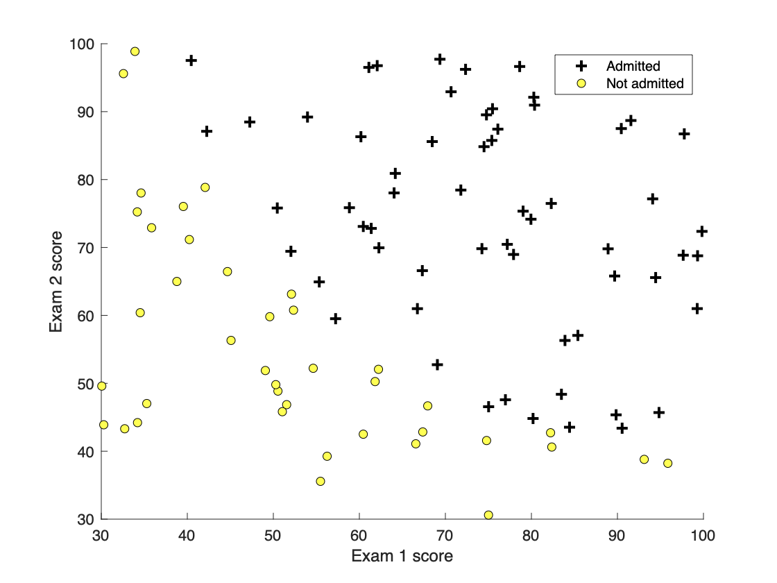
2.1 Part 1: Plotting mapping

Data set meaning ： The dataset has 100 Student's two exam results （ Deposit in X in ）, It is proposed to use logistic regression （ A dichotomous model ）, Estimate the admission probability of each student （ Admission indicates output y by 1, On the contrary, output y by 0）.
Matlab

 The main function 
%  Extract the data 
data = load(‘ex2data1.txt’);
X = data(:, [1, 2]); y = data(:, 3);
%  Load sub functions plotData
plotData(X, y);
%  Set up x、y Axis 
hold on;
% Labels and Legend
xlabel(‘Exam 1 score’)
ylabel(‘Exam 2 score’)
%  Add legend 
legend(‘Admitted’, ‘Not admitted’)
hold off;

plotData.m

pos = find(y==1); neg = find(y==0);
plot(X(pos, 1),X(pos,2), 'k+', 'LineWidth', 2, 'markersize',7);
plot(X(neg, 1),X(neg,2), 'ko', 'MarkerFaceColor', 'y');

2.2 Part 2: Compute Cost and Gradient Calculation cost and gradient

 The main function 
%  Deposit in X The line of / Number of columns 
[m, n] = size(X);
%  initialization X、theta
X = [ones(m, 1) X];
initial_theta = zeros(n + 1, 1);
% Compute and display initial cost and gradient
[cost, grad] = costFunction(initial_theta, X, y);
% Compute and display cost and gradient with non-zero theta
test_theta = [-24; 0.2; 0.2];
[cost, grad] = costFunction(test_theta, X, y);

computeCost.m

J = (1/m)*(-y'*log(sigmoid(X*theta))-(1-y)'*log(1-sigmoid(X*theta)));
grad =(1/m)*X'*(sigmoid(X*theta)-y);

2.3 Part 3: Optimizing using fminunc utilize fminuc Function optimization

No code is required for this section , according to fminuc Functions and plot Function to draw the decision boundary line .

2.4 Part 4: Predict and Accuracies Prediction and accuracy calculation

 The main function 
prob = sigmoid([1 45 85] * theta);
p = predict(theta, X);
fprintf(‘Train Accuracy: %f\n’, mean(double(p == y)) * 100);

predict.m

G =sigmoid(X*theta);
for i= 1 :m
    if G(i)<0.5
        G(i)=0;
    else
        G(i)=1;
    end
end

ex2 The logical regression of regularization

Practical significance ： I have a batch of chips tested twice and whether they are qualified or not , Hope to build a logistic regression model , According to the test data of the new chip, we can predict whether it is qualified or not .

3.1 Part 1: Regularized Logistic Regression Regularized logistic regression

First, data falsification , Secondly, the regularization coefficient is loaded $\lambda$ The cost function of , Get the picture below ：

When the decision boundary is no longer a straight line , You need a complex polynomial to represent , And as the polynomial becomes more complex , The higher the degree of fit , The over fitting phenomenon will be achieved , In this case, regular terms can be added to make use of $\lambda$ To reduce $\theta$ The effect of parameters .
$$J(\theta )=\frac{1}{m}\sum _{i=1}^m[-y^{(i)}log(h_{\theta }(x^{(i)}))-(1-y^{(i)})log(1-x^{(i)}))]+\frac{\lambda }{2m}\sum _{i=1}^m{\theta }_j^{(i)}$$

costFunctionReg.m

theta_1 =[0;theta(2:end)];
reg=lambda/(2*m)*theta_1'*theta_1;
J=1/m*(-y'*log(sigmoid(X*theta))-(1-y)'*log(1-sigmoid(X*theta)))+reg;
grad=1/m*X'*(sigmoid(X*theta)-y)+lambda/m*theta_1;

3.2 Part 2: Regularization and Accuracies Regularization and accuracy

Similar to the above logistic regression , adopt fminunc Get the minimum cost function theta value , Draw the decision boundary on the graph .

3.3 Compare different regularization parameters

$lambda=0$

$lambda=100$

From this we can get the appropriate $lambda$ It can effectively avoid the over fitting problem and ensure the fitting degree of the test set data .

---

Reference article ：
Machine learning programming assignments ex2(matlab/octave Realization )- Wu enda coursera
Matlab Wuenda machine learning programming practice ex2： Logical regression Logistic Regression