【sklearn】PCA

sklearn.decomposition.PCA

import matplotlib.pyplot as plt
from sklearn.datasets import load_iris
from sklearn.decomposition import PCA

iris = load_iris()
X = iris.data
Y = iris.target
# 二维数组，四维特征矩阵
X.shape 
(150, 4)

PCA()使用

# 默认降维到min(X.shape)
pca = PCA(n_components=2) # 降到2维
pca = pca.fit(X)
X_dr = pca.transform(X)
# X_dr = PCA(2).fit_transform(X)
X_dr.shape
 (150, 2)

# 降维到2维后，方便画图查看样本分布
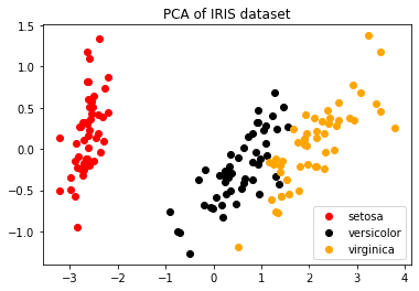
plt.figure()
plt.scatter(X_dr[Y==0, 0], X_dr[Y==0, 1], c='red', label=iris.target_names[0])
plt.scatter(X_dr[Y==1, 0], X_dr[Y==1, 1], c='black', label=iris.target_names[1])
plt.scatter(X_dr[Y==2, 0], X_dr[Y==2, 1], c='orange', label=iris.target_names[2])
plt.title('PCA of IRIS dataset')
plt.legend()
plt.show()
# 越近越相似，很适合KNN等聚类模型

# 查看新特征向量的信息量大小(可解释性方差)
print(pca.explained_variance_)
# 查看新特征向量的信息量占原始数据信息量的百分比(可解释性方差贡献率)
print(pca.explained_variance_ratio_)
# 降维后保留的信息量
print(pca.explained_variance_ratio_.sum())
''' [4.22824171 0.24267075] [0.92461872 0.05306648] 0.9776852063187949 '''

累积可解释方差贡献率曲线

pca_line = PCA().fit(X)
print(pca_line.explained_variance_ratio_)
 [0.92461872 0.05306648 0.01710261 0.00521218]
''' 降到1维保留0.92461872， 降到2维保留0.92461872+0.05306648 降到4维保留1 array([0.92461872, 0.05306648, 0.01710261, 0.00521218]) '''
import numpy as np
# np.cumsum(pca_line.explained_variance_ratio_) # 累加
plt.plot([1,2,3,4], np.cumsum(pca_line.explained_variance_ratio_))
plt.xticks([1,2,3,4]) # 限制坐标轴显示整数
plt.xlabel('number of components after dimention reduction')
plt.ylabel('cumulative explained variance ratio')
plt.show()

n_components=‘mle’ 自选

# 最大似然估计(mle)自选超参数
# 计算量大
pca_mle = PCA(n_components='mle')
pca_mle = pca_mle.fit(X)
X_mle = pca_mle.transform(X)
print(pca_mle.explained_variance_ratio_)
 [0.92461872 0.05306648 0.01710261]
# 可见降至3维最佳

按信息量占比选超参数 SVD

''' 可通过尝试，选定要降至的维度 规定降维后信息保留0.97,添加svd_solver='full' svd奇异值分解(solver求解器) auto 自动按数据量选择full或randomized full 适合数据量不大 randomized 适合特征矩阵巨大 arpack (一般auto,算不出来randomized) '''
pca_f = PCA(n_components=0.97, svd_solver='full')
pca_f = pca_f.fit(X)
X_f = pca_f.transform(X)
print(pca_f.explained_variance_ratio_)
 [0.92461872 0.05306648]