论文阅读 (50)：A Novel Matrix Game with Payoffs of Maxitive Belief Structure

0 引入

0.1 题目

  IJIS2019：最大确信结构收益的矩阵博弈 (A novel matrix game with payoffs of maxitive belief structure)

0.2 背景

  最大确信结构 (maxitive belief structures，MBSs) 以一种特定的结构来表示不精确和不确定 (imprecise and uncertain) 信息，使其能够同时建模概率的非特异性和不精确性 (nonspecificity and imprecise)。

0.3 方法

  所提出的模型可用于描述博弈双方之间的相互作用，并提出了一种通过达到均衡点来求解的有效方法。

0.4 Bib

@article{
    Han:2019:690706,
author		=	{
    Yu Zhen Han and Yong Deng},
title		=	{
    A novel matrix game with payoffs of maxitive belief structure},
journal		=	{
    International Journal of Intelligent Systems},
volume		=	{
    34},
number		=	{
    4},
pages		=	{
    690--706},
year		=	{
    2019},
doi			=	{
    10.1002/int.22072}
}

1 基础知识

1.1 Dempster‐Shafer (D‐S) 置信理论

  为了处理不确定性，许多数学工具被相继提出，例如D数、Z数，以及模糊集。D-S置信理论也称为D-S理论或者置信理论，是由Dempster提出并被Shafer扩展。D-S理论可以被认为是贝叶斯概率理论的推广，因为它所需满足的约束比贝叶斯理论更弱。如今，D-S理论由于其可以处理不精确和不确定信息的能力，已被用在诸如信息融合、多边决策 (MCDM)、模式识别，以及风险分析等多种领域。以下介绍一些该理论的基本概念：
  定义1：辨别框架 (Frame of discernment) 令$\Omega =\{{\theta }_1,{\theta }_2,\dots ,{\theta }_n\}$表示包含$n$个元素的有限集，以及$P(\Omega )$表示包含$2^N$个元素的幂集：
$$P(\Omega )=\{\varnothing ,\{{\theta }_1\},\{{\theta }_2\},\dots ,\{{\theta }_n\},\{{\theta }_1,{\theta }_2\},\{{\theta }_1,{\theta }_3\},\Omega \}.\text{\hspace{1em}(1)}$$  定义2：基准概率分配 (Basic probability assignment, BPA) 幂集$P(\Omega )$到数值$0$-$1$之间的映射：
$$m:P(\Omega )\to [0,1],\text{\hspace{1em}(2)}$$其满足以下条件：
$$m(\varnothing )=0,\sum _{A\subseteq P(\Omega )}m(A)=1.\text{\hspace{1em}(3)}$$  这里$m(A)$表示实际应用中A的置信度。
  定义3：确信与合理性函数 (Belief and plausibility functions) 确信函数被定义为：
$$\text{Bel}:P(\Omega )\to [0,1]\text{ and Bel}(A)=\sum _{B\subseteq A}m(B),\text{\hspace{1em}(4)}$$合理性函数Pl被定义为
$$\text{Pl}:P(\Omega )\to [0,1]\text{ and Pl(A)}=\sum _{B\cap A\ne \varnothing }m(B)=1-\text{Bel}(\overline{A})\text{\hspace{1em}(5)}$$  $\text{Bel}(A)$和$\text{Pl}(A)$分别表示下界与上界。
  定义4：Dempster结合律 (Dempster combination rule) 如果$m(A)>0$，则$A$称为一个焦点元素 (focal element) ，所有焦点元素的集合称为证据体 (body of evidence, BOE)。当多个独立的BOEs可用时，可用使用Dempster结合律获取组合证据 (combined evidence)：
$$m(A)=\frac{\sum _{B,C\subseteq \Omega ,B\cap C=A}{m}_1(B)m_2(C)}{1-K},\text{\hspace{1em}(6)}$$其中$K={\sum }_{B\cap C=\varnothing }{m}_1(B)m_2(C)$是一个叫做冲突 (conflict) 的标准化常量。该结合律只有当$m_{\oplus }(\varnothing )\ne 1$时有意义；否则这些证据呈现总体对抗，该结合律失效，如何处理这些冲突将是一个开放性问题。

1.2 最大确信结构MBS的定义

  与变量$V$相关联的有限空间$X=\{x_1,x_2,\dots ,x_n\}$上的最大确信结构$M$由$X$的$q$个非空子集组成，称为焦点元素，表示为$F_i，i=1,2,\dots ,n$，其权重满足$M(F_i)\ge 0$且${\max }_{i}M(F_i)=1$。与经典D-S置信理论相比，焦点元素之和并不必要等于1，因此它可以更好的适配现实应用。
  假设$A$是$X$的一个子集，两个与$M$相关的，分别称为上界概率 (upper possibility) 和下届概率 (lower possibility) 重要集合函数定义如下：
$$\begin{array}{rl}{U}_M(A)& =\underset{i,A\cap F_i\ne \varnothing }{\max }\left\{M\left(F_i\right)\right\},\\ L_M(A)& =\underset{i,F_i\subseteq A}{\max }\left\{M\left(F_i\right)\right\}.\end{array}$$进一步可以将其表示为
$$\begin{array}{rl}{U}_M(A)& =\underset{i}{\max }\left[M\left(F_i\right)\wedge G_i(A)\right],\\ L_M(A)& =\underset{i}{\max }\left[M\left(F_i\right)\wedge H_i(A)\right],\end{array}$$其中如果$A\cap F_i\ne \varnothing$，$G_i(A)=1$否则等于$0$；如果$F_i\subseteq A$，则$H_i(A)=1$否则等于$0$。此外，$G_i(A)={\max }_i[F_i(x_i)\wedge A(x_i)]$，其中$F_i(x_i)$和$A(x_i)$是指示函数。$H_i(A)$同样可以被重写为：
$$H_i(A)=1-\underset{i}{\max }[F_i(x_i)\wedge (1-A(x_i))].\text{\hspace{1em}(9)}$$如果$A\cap F_i\ne \varnothing$，则$G_i(A)=1$否则$=0$；如果$F_i\in A$，则$H_i(A)=1$否则$=0$。
  定义5：MBS结合律 (Fusing rules of MBS) 假设$M_1$和$M_2$是两个提供了变量$V$信息的两个MBS，且它们各自的焦点元素分别为$F_1,F_2,\dots ,F_n$和$E_1,E_2,\dots ,E_q$。它们的结合规则可以定义如下：
$$M(F_i\cap E_j)=\frac{\min [M_1(F_i),M_2(E_j)]}{k}对于F_i\cap E_j\ne \varnothing .\text{\hspace{1em}(10)}$$其中$k={\max }_{F_i\cap E_j\ne \varnothing }\min [M_1(F_i),M_2(E_j)]$。这个操作可以被表示为$M=M_1\perp M_2$，其意味着最大融合。注意$\perp$具有对称性，即$M_1\perp M_2=M_2\perp M_1$。$k$是冲突系数，当$k=0$时，两个MBS总是冲突的，因此不能合并它们。如果存在$F^{\ast }$和$E^{\ast }$使得$M_1(F^{\ast })\cap M_2(E^{\ast })\ne \varnothing$和$M_1(F^{\ast })=M_2(E^{\ast })=1$，则
$$M(F_i\cap E_j)=\min [M_1(F_i),M_2(E_j)]对于F_i\cap E_j\ne \varnothing .\text{\hspace{1em}(11)}$$可以很容易地证明$k$是一个折扣系数 (discounting coefficient) 且$\max M(F)=1$。进一步，公式11可以被扩展到更多MBS的情况。假设$M_i,i=1,2,\dots ,n$是包含焦点元素$F_{ij}$的多个MBS。当条件$F_{1j_1}\cap F_{2j_2},\dots ,\cap F_{n{j}_n}\ne \varnothing$满足时，有
$$M\left(F_{1j_1}\cap F_{2j_2},\dots ,\cap F_{n{j}_n}\right)=\frac{\min \left[M_1\left(F_{1j_1}\right),M_2\left(F_{2j_2}\right),\dots ,M_n\left(F_{n{j}_n}\right)\right]}{k},\text{\hspace{1em}(12)}$$其中当$M_i$是一个纯概率分布时，有$k={\max }_{F_{1j}\cap F_{2j},\dots ,\cap F_{nj}\ne \varnothing }\min \left[M_1\left(F_{1j_1}\right),M_2\left(F_{2j_2}\right),\dots ,M_n\left(F_{n{j}_n}\right)\right]$。

2.3 具有清晰数字收益的传统矩阵博弈 (Traditional matrix game with crisp number payoffs)

  一场博弈中通常包含多个玩家的集合以及每个玩家的有限策略集合。令$S_{A1}=\{s_{A1},s_{A2},\dots ,s_{Am}\}$和$S_{B1}=\{s_{B1},s_{B2},\dots ,s_{Bn}\}$表示玩家$A$和玩家$B$的纯粹策略集合。令$A=\{a_1,a_2,\dots ,a_m\}$和$B=\{b_1,b_2,\dots ,b_n\}$表示玩家$A$和$B$的混合策略。令$X=(x_{ij}{)}_{m\times n}$表示$A$的支付矩阵 (payoff matrix) ，则三元组$(\{A\},\{B\},X)$可以表示两个玩家的零和矩阵博弈：
$$AX{B}^T=\sum _{i=1}^m\sum _{j=1}^n{a}_i{x}_{ij}{b}_j.\text{\hspace{1em}(13)}$$这种情况下，玩家$B$的期望损失则是$-AX{B}^T$。
  John von Neumann证明了最小最大定理 (minimax theorem) 可以处理矩阵博弈问题，从而找到玩家双方的理想策略。证明现实，玩家应该寻求使自身的最小预期收益最大化的混合策略，或者玩家应该优先考虑使自身预期最大损失最小的混合策略。这个理论可以描述为一个线性规划 (linear programming) 问题：
  $\max u$
$$\text{ s.t. }\{\begin{array}{l}{\sum }_{i=1}^m{x}_{ij}{a}_i\ge u,j=1,2,\dots ,n,\\ {\sum }_{i=1}^m{a}_i=1\\ a_i\ge 0,i=1,2,\dots ,m\end{array}\text{\hspace{1em}(14)}$$
且$\min v$
$$\text{ s.t. }\{\begin{array}{l}{\sum }_{i=1}^n{x}_{ij}{b}_i\le v,j=1,2,\dots ,m,\\ {\sum }_{i=1}^n{b}_i=1,\\ b_i\ge 0,i=1,2,\dots ,n.\end{array}\text{\hspace{1em}(15)}$$公式14和15实际上是原始对偶线性规划问题，这意味着$u$的最大值等于$v$的最小值。值$Z=u=v$便是矩阵博弈的解。
  以下使用一个例子来更清晰的认识如何使用最小最大定理求解矩阵博弈。令$(S_A,S_B,X)$表示当前博弈，其中玩家$A$有三个策略，即$S_A=\{s_{A1},s_{A2},s_{A3}\}$，玩家$B$有四个策略，即$S_B=\{s_{B1},s_{B2},s_{B3},s_{B4}\}$。玩家$A$的支付矩阵为：
$$A=\left(\begin{array}{rrrr}5& 6& -8& -5\\ -5& 8& 10& -4\\ 7& 5& -10& 9\end{array}\right)$$  在零和博弈中，玩家$B$的支付矩阵为$-A$。令$A=\{a_1,a_2,a_3\}$和$B=\{b_1,b_2,b_3,b_4\}$分别表示玩家$A$和$B$的混合策略。博弈的平衡 (equilibrium) 或者说结果可以通过公式14和15获取：
  $\max u$
$$\text{ s.t. }\{\begin{array}{l}5a_1-5a_2+7a_3\ge u,\\ 6a_1+8a_2+5a_3\ge u,\\ -8a_1+10a_2-10a_3\ge u,\\ -5a_1-4a_2+9a_3\ge u,\\ a_1+a_2+a_3=1,\\ a_1,a_2,a_3\ge 0\end{array}$$且$\min v$
$$\text{ s.t. }\{\begin{array}{l}5b_1+6b_2-8b_3-5b_4\le v\\ -5b_1+8b_2+10b_3-4b_4\le v\\ 7b_1+5b_2-10b_3+9b_4\le v\\ b_1+b_2+b_3+b_4=1\\ b_1,b_2,b_3,b_4\ge 0\end{array}\text{\hspace{1em}(16)}$$  通过优化求解，平衡将在$A^{\ast }=(0,0.5312,0.4687)$和$B^{\ast }=(0.625,0,0.3750,0)$达到。此时有$u=v=0.6250$。

3 基于MBS的矩阵博弈

  本节提出了一个具有MBS收益的矩阵博弈，其同时考虑不和谐 (discord) 和非特异性 (nonspecificity)。以下首先给出一些定义：
  定义6： 玩家$A$偏好策略$A$，玩家$B$偏好策略$B$，可以将其简写为：
$${\mathrm{MG}}_{\text{MBS}}=(A,B,X),$$其中$X=(M_{ij}{)}_{m\times n}$是玩家A的MBS支付矩阵。因此$X$的每个元素$M_{ij}$都是一个MBS，其受到辨别框架$\Omega =\{{\theta }_1,{\theta }_2,\dots ,{\theta }_n\}$的约束。
  根据定义6，$M_{ij}$表示玩家$A$采用纯粹策略$S_{Ai}$且玩家$B$采用纯粹策略$S_{Bj}$时的增益 (gain)。该增益由$\Omega$上的MBS表示。对于博弈矩阵中包含的非特异性和不和谐，评价等级${\theta }_1,{\theta }_2,{\theta }_n$可以是线性语言变量 (linear linguistic variables)，从而将不确定性包含在博弈中。此外，在采用混合策略的情况下，例如玩家$A$偏好混合策略$A$，玩家$B$偏好混合策略$B$，则玩家$A$的期望增益可以记作$M_{xy}$，且可以通过矩阵博弈${\text{MG}}_{\text{MBS}}$中的以下等式计算：
$$M_{AB}(A)=\sum _{i=1}^m\sum _{j=1}^n{a}_i{b}_j{M}_{ij}(A),A\in \Omega .\text{\hspace{1em}(17)}$$一旦零和博弈中的MBS结构支付矩阵被矩阵，便可以通过以下步骤计算平衡。

3.1 阶段1：决定辨别框架的相对效应

  在${\text{MG}}_{\text{MBS}}$中，支付矩阵通过MBS表示。然而MBS却是无法量化的。在博弈中，效用的增加或减损是通过矩阵博弈中玩家的得失来衡量的。在这种场景下，我们通过量化效用的改变来调整MBS。目前$\Omega$两两元素之间的相对相应已经定义，为了简化效用函数的形式，一个链式效用函数 (chain utility function) 被定义如下：
$$u({\theta }_i)=f_{i,i-1}(u({\theta }_{i-1})),2\le i\le n,\text{\hspace{1em}(18)}$$其中$u({\theta }_i)$是${\theta }_i$的效用。根据公式9，如果$\Omega$的大小是$n$，则$n-1$项应当被考虑。基于此，可以获取任意两个元素的相对效用。

3.2 步骤2：消除非特异性和不和谐

  在MBS中，非特异性和不和谐这两种不确定性应当被考虑，然后同时对它们进行处理是困难的。对此，我们基于理想情况与极端情况来消除支付矩阵的不确定性。MBS的效用可以被表示为$$u\left(M_{ij}\right)=\left[u_{ij}^L,u_{ij}^R\right]\text{\hspace{1em}(19)}$$其中
$$\{\begin{array}{l}{u}_{ij}^L={\sum }_{\theta \in \Omega }{U}_M(\theta )u(\theta )={\sum }_{\theta \in \Omega }{\max }_{i,\theta \cap F_i\ne \varnothing }\left\{M\left(F_i\right)\right\}u(\theta ),\\ u_{ij}^R={\sum }_{\theta \in \Omega }{L}_M(\theta )u(\theta )={\sum }_{\theta \in \Omega }{\max }_{i,F\in \Theta \in }\left\{M\left(F_i\right)\right\}u(\theta ).\end{array}\text{\hspace{1em}(20)}$$  中间值支付矩阵 (interval-valued payoff matrix) 可以计算为：
$$U=u(M)={\left(\left[u_{ij}^L,u_{ij}^R\right]\right)}_{m\times n}.\text{\hspace{1em}(21)}$$

3.3 步骤3：计算平衡点

  一些已有的方法可以用于处理${\text{MG}}_{\text{MBS}}$所转换的中间值矩阵博弈：
  $\max \overline{u}$
$$\text{ s.t. }\{\begin{array}{l}{\sum }_{i=1}^m{u}_{ij}{a}_i\ge \bar{u},j=1,2,\dots ,n,\\ u_{ij}^L\le u_{ij}\le u_{ij}^R\\ {\sum }_{i=1}^m{a}_i=1,\\ a_i\ge 0,i=1,2,\dots ,m\end{array}\text{\hspace{1em}(22)}$$
且$\min \underline{v}$
$$\text{ s.t. }\{\begin{array}{l}{\sum }_{i=1}^n{u}_{ij}{b}_i\le \underline{v},j=1,2,\dots ,m\\ u_{ij}^L\le u_{ij}\le u_{ij}^R\\ {\sum }_{i=1}^n{b}_i=1\\ b_i\ge 0,i=1,2,\dots ,n.\end{array}\text{\hspace{1em}(23)}$$
以上公式可以转换为以下的两个线性规划：
  $\max \bar{u}$
$$\text{ s.t. }\{\begin{array}{l}{\sum }_{i=1}^m{u}_{ij}^R{a}_i\ge \bar{u},j=1,2,\dots ,n\\ {\sum }_{i=1}^m{a}_i=1\\ a_i\ge 0,i=1,2,\dots ,m\end{array}\text{\hspace{1em}(24)}$$
且$\min \underline{v}$
$$\text{ s.t. }\{\begin{array}{ll}{\sum }_{i=1}^n& u_{ij}^L{b}_i\le \underline{v},j=1,2,\dots ,m\\ {\sum }_{i=1}^n& b_i=1\\ b_i\ge 0,& i=1,2,\dots ,n.\end{array}\text{\hspace{1em}(25)}$$  根据线性规划的对偶理论，以上公式可以被进一步转换为：
  $\min \bar{v}$
$$\text{ s.t. }\{\begin{array}{l}{\sum }_{i=1}^m{u}_{ij}^R{b}_i\le \bar{v},j=1,2,\dots ,m,\\ {\sum }_{i=1}^m{b}_i=1,\\ a_i\ge 0,i=1,2,\dots ,n\end{array}\text{\hspace{1em}(26)}$$
且$\max \underline{u}$
$$\text{ s.t. }\{\begin{array}{ll}{\sum }_{i=1}^n& u_{ij}^L{b}_i\ge \underline{u},j=1,2,\dots ,n,\\ {\sum }_{i=1}^n& a_i=1,\\ b_i\ge 0,& i=1,2,\dots ,m.\end{array}\text{\hspace{1em}(27)}$$  通过求解线性规划问题，可以获取获取平衡$({\overline{a}}^{\ast },{\overline{b}}^{\ast })$和$({\underline{a}}^{\ast },{\underline{b}}^{\ast })$，其分别对应于公式24、26、27，以及15的解。

3.4 求解${\text{MG}}_{\text{MBS}}$的值

  本节对${\text{MG}}_{\text{MBS}}$上的值进行形式化定义：
  定义7：令${\text{MG}}_{\text{MBS}}=(A,B,X)$表示矩阵博弈，$({\overline{a}}^{\ast },{\overline{b}}^{\ast })$和$({\underline{a}}^{\ast },{\underline{b}}^{\ast })$是矩阵平衡点，则${\text{MG}}_{\text{MBS}}$中的值是$V=[V^L,V^R]$，其满足
$$\begin{array}{rl}{V}^L=u_{{\underline{a}}^{\ast }{\underline{b}}^{\ast }}& =\sum _{\theta \in \Omega }{U}_M(\theta )u(\theta )=\sum _{\theta \in \Omega }\underset{i,\theta \cap F\ne \varnothing }{\max }\left\{M\left(F_i\right)\right\}u(\theta ),\\ V^R=u_{{\tilde{a}}^{\ast }{\dot{b}}^{\ast }}& =\sum _{\theta \in \Omega }{L}_M(\theta )u(\theta )=\sum _{\theta \in \Omega }\underset{i,F_i\subseteq \theta }{\max }\left\{M\left(F_i\right)\right\}u(\theta ).\end{array}\text{\hspace{1em}(28)}$$最终，玩家$A$的预期平衡收益或者玩家$B$的预期平衡损失可以通过${\text{MG}}_{\text{MBS}}$呈现，其值便是MBS中非特异性和不和谐的体现。此外，当$M_{{\overline{a}}^{\ast }{\overline{b}}^{\ast }}=$$M_{{\underline{a}}^{\ast }{\underline{b}}^{\ast }}$$=M_{a^{\ast }{b}^{\ast }}$，${\text{MG}}_{\text{MBS}}$的值可以表示为$V=M_{a^{\ast }{b}^{\ast }}$。

4 事件分析

  本节通过领土争端问题来验证所提出的具有MBS收益矩阵博弈的有效性和有效性。领土主权不可分割，可以说是一场零和博弈。 如图1所示，名为ALPHA和BETA的两个国家同时争夺领土Zeta。由于这两个国家处于战争边缘，联合国派出专家组评估一些可行的政策来缓解两国的压力。

图1：领土争端问题

4.1 博弈分析

  这一步通过分析ALPHA和BETA两国的历史决策和行为来评估它们可能采用的潜在策略。这种情况下，假设ALPHA有三个可能的策略而BETA有四个可能的策略。
  ALPHA的策略如下：
  1）$S_{A1}$：与BETA谈判并作出一些妥协；
  2）$S_{A2}$：分配更多的兵力到Zeta；
  3）$S_{A3}$：采取一些负面策略。
  BETA的策略如下：
  1）打仗；
  2）局部冲突；
  3）福利政策
  4）军事对抗。

4.2 决策分析

  由于多变环境下存在不精确性和不确定性，不同策略组合下的收益无法确定为一个准确的数字。因此，MBS被用来表述不确定支付。为了简单地代表从专家那里收集的评估，评估等级首先使用辨别框架$\Omega$来确定。具体地，值为不确定信息的语言变量构成辨别框架：
$$\Omega =\{\text{Very Bad }(VB),\text{Bad }(B),\text{Fair }(F),\text{Good }(G),\text{Very Good }(VG)\}.$$  一旦辨别框架中的语言变量确定，则应指任何一对语言变量之间的相对效用，以将它们限制在统一标准中。在这个例子中，考虑到$\Omega$的大小为$5$，我们设置了$10$个效用关系，即固定一组相对效用函数来描述语言变量之间的效用关系，如下所示：
$$U(VG)/U(G)=2,U(G)/U(F)=2,U(F)/U(B)=2,U(B)/U(VB)=2.\text{\hspace{1em}(29)}$$

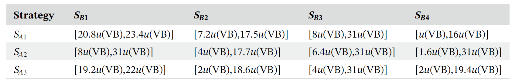
4.3 支付评估

  博弈中的支付矩阵可以根据语言评估和玩家策略进行构建。由于该博弈是零一博弈，仅有ALPHA或者BETA的支付矩阵被给定。表1展示的是ALPHA的支付矩阵，需要注意的是每一个评估都被表示为MBS的结构，以表达非特异性和不和谐。

表1：ALPHA的支付矩阵

4.4 求解MBS矩阵博弈

  首先，通过公式20可以消除非特异性和不和谐，MBS矩阵博弈可以被转换为中间值支付矩阵，如表2。

表2：ALPHA的中间值支付矩阵

  然后，基于公式29，我们将表2转换成只包含$u(VB)$的形式，如表3。

表3：ALPHA只包含VB的支付矩阵

  再者，表3中的支付矩阵可以被转换为两个清晰的支付矩阵$U^L$和$U^R$：
$$\begin{array}{c}{U}^L=\left[\begin{array}{cccc}20.8u(\mathrm{V}\mathrm{B})& 7.2u(\mathrm{V}\mathrm{B})& 8u(\mathrm{V}\mathrm{B})& 1u(\mathrm{V}\mathrm{B})\\ 8u(\mathrm{V}\mathrm{B})& 4u(\mathrm{V}\mathrm{B})& 6.4u(\mathrm{V}\mathrm{B})& 1.6u(\mathrm{V}\mathrm{B})\\ 19.2u(\mathrm{V}\mathrm{B})& 2u(\mathrm{V}\mathrm{B})& 4u(\mathrm{V}\mathrm{B})& 2u(\mathrm{V}\mathrm{B})\end{array}\right],\\ U^R=\left[\begin{array}{cccc}23.4u(\mathrm{V}\mathrm{B})& 17.5u(\mathrm{V}\mathrm{B})& 31u(\mathrm{V}\mathrm{B})& 16u(\mathrm{V}\mathrm{B})\\ 31u(\mathrm{V}\mathrm{B})& 17.7u(\mathrm{V}\mathrm{B})& 31u(\mathrm{V}\mathrm{B})& 31u(\mathrm{V}\mathrm{B})\\ 22u(\mathrm{V}\mathrm{B})& 18.6u(\mathrm{V}\mathrm{B})& 31u(\mathrm{V}\mathrm{B})& 19.4u(\mathrm{V}\mathrm{B})\end{array}\right].\end{array}$$  对于$U^L$，根据章节3有
$\max \underline{u}$
$$\text{ s.t. }\{\begin{array}{l}20.8a_1+8a_2+19.2a_3\ge \underline{u}\\ 7.2a_1+4a_2+2a_3\ge \underline{u}\\ 8a_1+6.4a_2+4a_3\ge \underline{u}\\ 1a_1+1.6a_2+2a_3\ge \underline{u}\\ a_1+a_2+a_3=1\\ a_1,a_2,a_3\ge 0\end{array}$$
且$\min \underline{v}$
$$\text{ s.t. }\{\begin{array}{l}20.8b_1+7.2b_2+8b_3+b_4\le \underline{v}\\ 8b_1+4b_2+6.4b_3+1.6b_4\le \underline{v}\\ 19.2b_1+2b_2+4b_3+2b_4\le \underline{v}\\ b_1+b_2+b_3+b_4=1\\ b_1,b_2,b_3,b_4\ge 0\end{array}$$  可以求得对于$U^L$，最优解为${\underline{a}}^{\ast }=(0,0,1)$以及${\underline{b}}^{\ast }=(0,0.0618,0,0.9382)$。
  同理对于$U^R$有
$\max \bar{u}$
$$\text{ s.t. }\{\begin{array}{l}23.4a_1+31a_2+22a_3\ge \bar{u}\\ 17.5a_1+17.7a_2+18.6a_3\ge \\ 31a_1+31a_2+31a_3\ge \bar{u}\\ 16a_1+31a_2+19.4a_3\ge \bar{u}\\ a_1+a_2+a_3=1\\ a_1,a_2,a_3\ge 0\end{array}$$
且$\min \bar{v}$
$$\text{ s.t. }\{\begin{array}{l}23.4b_1+17.5b_2+31b_3+16b_4\le \bar{v}\\ 31b_1+17.7b_2+31b_3+31b_4\le \bar{v}\\ 22b_1+18.6b_2+31b_3+19.4b_4\le \bar{v}\\ b_1+b_2+b_3+b_4=1\\ b_1,b_2,b_3,b_4\ge 0\end{array}$$此时的最优解为${\overline{a}}^{\ast }=(0,0,1)$以及${\overline{b}}^{\ast }=(0,1,0,0)$。因此，ALPHA的期望收益可以通过公式14获得。
  在平衡点$({\underline{a}}^{\ast },{\underline{b}}^{\ast })$有：
$$M(B)=1.$$  在平衡点$({\overline{a}}^{\ast },{\overline{b}}^{\ast })$有：
$$M(VG)=0.6,M(G)=0.6,M(F)=0.4,M(B)=1,M(VB)=0.6.$$  最终，MBS矩阵博弈的值便是$[\min u(M_{{\underline{a}}^{\ast }{\underline{b}}^{\ast }}),\max u(M_{{\overline{a}}^{\ast }{\overline{b}}^{\ast }})]$$=[u(B),0.6u(VG)+0.6u(G)+0.4u(F),u(B)+0.6u(VB)]$。