[paper reading ｜ deep reading] drne:deep recursive network embedding with regular equivalence

Preface

Hello！
Thank you very much for reading Haihong's article , If there are mistakes in the text , You are welcome to point out ～
 
Self introduction. ଘ(੭ˊᵕˋ)੭
nickname ： Sea boom
label ： Program the ape ｜C++ player ｜ Student
brief introduction ： because C Language and programming , Then I turned to computer science , Won a National Scholarship , I was lucky to win some national awards in the competition 、 Provincial award … It has been insured .
Learning experience ： Solid foundation + Take more notes + Knock more code + Think more + Learn English well ！
 
Only hard work
 

Know what it is Know why ！

 
This article only records what you are interested in

ABSTRACT

The purpose of network embedding is to embed in the embedded space Maintain vertex similarity

The existing methods usually define similarity through the direct connection or common neighborhood between nodes , namely Structural equivalence

However , Vertices in different parts of the network may have similar roles or positions , That is, regular equivalence , This point is basically ignored in the network embedded literature .

Regular equivalence is defined recursively , That is, two regular equivalent vertices have the same regular equivalent network neighbors .

therefore , We propose a new deep recursive network embedding method to learn network embedding with rule equivalence .

More specifically , We propose a layer normalized LSTM, Each node is represented by recursively aggregating their neighborhood representations .

We theoretically proved some popular 、 Typical 、 The centrality measure conforming to the rule equivalence is the optimal solution of our model .

1 INTRODUCTION

There are many ways to quantify the similarity of vertices in a network . The most common is structural equivalence [18].

If two vertices share many of the same network neighbors , Then they are structurally equivalent .

In the past, most of the researches on network embeddedness aim at High order nearest neighbors to maintain structural equivalence [33,35]

Expand the network neighborhood to high-order nearest neighbor , Such as immediate neighbors 、 A neighbor's neighbor, etc （ Nested loop ）.

However , in many instances , Vertices have similar roles or occupy similar positions , and There are no public neighbors . for example ：

The relationship pattern between two mothers and their husbands and several children is the same .
Although if two mothers do not have the same relatives , They are not structurally equal , But they do play similar roles or positions .

These cases lead us to the extended definition of vertex similarity , It is called regular equivalence .

If the network neighbors of two vertices are similar ( That is, rule equivalence ), Then they are defined as rule equivalence

obviously , Rule equivalence is a relaxation of structural equivalence . Structural equivalence guarantees rule equivalence , But the opposite is not true .

by comparison , Rule equivalence is more flexible , It can cover a wide range of network applications related to the importance of structural roles or nodes , But to a large extent, it is ignored by the literature embedded in the network .

---

In order to maintain the regular equivalence in network embedding , That is, two regular equivalent nodes should have similar embeddedness .

One simple way is Explicitly compute the regular equivalence of all vertex pairs , The similarity of node embedding is required to approximate its corresponding regular equivalence .

But for large-scale networks , It's not feasible , Because the complexity of calculating rule equivalence is very high .

Another option is Replace the conventional equivalence with a simpler graph theoretic metric , For example, centrality measurement .

Although many centrality measures have been designed to characterize the role and importance of vertices , But a centrality can only capture specific aspects of network roles , This makes it difficult to learn general task independent node embedding . Not to mention some central metrics , Such as intermediate centrality , It also has high computational complexity

How to effectively embed in the network 、 Maintaining regular equivalence efficiently is still a problem to be solved .

---

As mentioned earlier , The definition of regular equivalence is recursive . It inspired us to Learn network embedding recursively , namely The embedding of a node is aggregated through the embedding of its neighbors

In a recursive step ( Pictured 1 Shown ), If node 3 and 5、4 and 6、7 and 8 Rule equivalence , So there is already a similar embedding , The node 1 and 2 Will have a similar embed , So that their rules are equivalent to true .

---

It's based on this idea , We propose a new deep recursive network embedding (DRNE) Method .

More specifically

• We convert the neighbors of nodes into an ordered sequence
• A layer normalization method is proposed LSTM
• The neighbor embedding is aggregated into the target node embedding in a nonlinear way .

We theoretically prove that some popular and typical centrality measures are the optimal solution of our model .

The experimental results also show that , The learned node representation can well maintain pairwise regular equivalence , And predict the values of multiple centrality measures for each node .

---

This paper has the following contributions :

• We study a new node representation learning problem with regular equivalence , This is a key problem in network analysis , However, it has been largely ignored in the literature of web-based learning .
• We find an effective method to integrate the global regular equivalent information into the node representation , A new deep model is proposed DRNE, The model learns node representation by recursively aggregating neighbor representations in a nonlinear manner .
• We prove theoretically that the learned node representation can keep pairwise regular equivalence well , It also reflects several popular and typical node centrality . The experimental results also show that , This method is obviously superior to centrality measurement and other network embedding methods in structural role classification .

2 RELATED WORK

Most of the existing network embedding methods are developed along the route of maintaining the observed pairwise similarity and structural equivalence .

• DeepWalk[28] Use random walk to generate a sequence of nodes from the network , The language model is used to learn node representation by treating sequences as sentences
• Node2vec[12] It extends this idea , A biased second-order random walk model is proposed
• LINE[33] An objective function is optimized , The purpose is to maintain the pairwise similarity and structural equivalence of nodes .
• M-NMF[36] Will be more macro structure —— The community structure is incorporated into the embedding method
• Structural Deep Network Embedding Claim that the underlying structure of the network is highly nonlinear , A model of depth self encoder is proposed , To maintain the first-order and second-order proximity of the network structure .
• Label informed attributed network embedding & Attributed network embedding for learning in a dynamic environment： Add node attributes to the network , Smoothly embed attribute information and topology into low dimensional representation
• RolX[13] Enumerate various handmade structural features for nodes , And find a more suitable basis vector for this joint feature space
• Similarly ,struc2vec[29] Structural similarity is measured by defining some form of centrality heuristic , The explicit computation of centrality similarity makes it not extensible

When learning to express , None of these methods can maintain rule equivalence

---

Rule equivalence is a relaxed concept of structural equivalence , Can better capture structural information

• REGE[7] and CATREGE[7] It is achieved by iteratively searching for the optimal match between two vertex neighbors
• VertexSim[18] Using the recursive method of linear algebra to construct the similarity measure . However, due to the high computational complexity of rule equivalence , This is not feasible in large-scale networks

---

Centrality measure It is another method to measure the node structure information in the network

In order to study how to better capture structural information , A set of centrality [3,20,21]
Because each of them captures only one aspect of the structure information , A certain centrality does not support different networks and applications well
Besides , The manual approach to design centric metrics makes them less comprehensive , It is not possible to include information about general equivalence

in summary , For learning node representations with rule equivalence , There is still no good solution

3 DEEP RECURSIVE NETWORK EMBEDDING

DRNE Overall frame diagram

• （a） Sampling neighborhood
• （b） Sort the nodes in the neighborhood （ According to the degree ）
• （c） Layer normalization LSTM, Aggregate the embeddedness of adjacent nodes into the embeddedness of target nodes .$X_i$ For the node i Embedding of ,$LN$ Normalize the layer
• （d） Weakly guided regularizer

---

Understanding of the steps in the figure ：

• （a） To the node 0 For example , Let's start with its neighbor node 123 sampling
• （b） Press degree Sort to form a sequence （312）
• （c） Use the domain sequence $X_3,X_2,X_1$ As the input , Through single layer normalized LSTM Get an integrated representation $h_T$ , adopt $h_T$ Reconstruct the embedded vector $X_0$ And nodes $0$, Embedded vector $X_0$ It can well preserve the local domain properties .
• （d） On the other hand , We can spend $d_0$ Weak supervisory information as a central measure , take $h_T$ Input to multilayer perceptron MLP in , To approximate $d_0$ . Perform the same process for other nodes in the network . When we update $X_3,X_1,X_2$ when , node $0$ Embedding of $X_0$ It will also be updated . Repeat the process by iterating over and over again , So embedded $X_0$ It can contain the organization information of the whole network

Reference resources ：https://zhuanlan.zhihu.com/p/104488503

3.1 Notations and Definitions

$G=(V,E)$

$N(v)=\{u|(v,u)\in E\}$

$\mathbf{X}={\mathbb{R}}^{|V|\times k}$： Embedded space vector representation of vertices

$d_v=|N(v)|$： The vertices $v$ Degree

$I(x)=\{\begin{array}{l}1x\ge 0\\ 0else\end{array}$

---

Definition 3.1 (Structural Equivalence)

• $s(u)=s(v)$ : node $u$ and $v$ Structural equivalence
• $N(u)=N(v)\Rightarrow s(u)=s(v)$
• That is, the neighborhood of nodes is the same , Is structurally equivalent

Definition 3.2 (Regular Equivalence)

• $r(u)=r(v)$： node $u$ and $v$ Is regular equivalence
• $\{r(i)|i\in N(u)\}=\{r(j)|j\in N(u)\}$（ Did not understand ）

3.2 Recursive Embedding

According to the definition 3.2, We learn node embedding recursively , The embedding of the target node can be approximated by the aggregation embedded by its neighbor nodes

Based on this concept , We design the following loss function :

among Agg It's an aggregate function

---

In a recursive step , The learned embedded node can retain the local structure of its neighbors

adopt Iteratively update the learned representation , The learned node embedding can In a global sense, the structural information is fused , This is consistent with the definition of rule equivalence

---

The underlying structure of real networks is often highly nonlinear [22], We designed a depth model , Normalized long-term and short-term memory layer (ln-LSTM)[2] As an aggregate function

as everyone knows ,LSTM Modeling sequences is effective . However , The neighbors of nodes do not have natural ordering in the network

Here we are The degree of nodes is used as a criterion to sort neighbors into an ordered sequence

• This is mainly because degree is the most effective measure of neighbor ranking
• Degree plays an important role in many graph theoretic measures , Especially those metrics related to structural roles , Such as PageRank[27] and Katz[25]

---

set up

• Ordered neighborhood The embedding of is $\{X_1,X_2,\dots ,X_t,\dots ,X_T\}$
• At each time step $t$ when , Cryptic state $h_t$ yes $t$ The input of time is embedded $X_t$ And its previous implicit state $h_{t-1}$ Function of , namely $h_t=LSTMCell(h_{t-1},X_t)$

When LSTM Cell The embedded sequence is transformed from 1 To T Recursive processing of , Implies $h_t$ The information will be more and more abundant

$h_T$ It can be seen as an aggregated representation of neighbors .

In order to learn the long-distance correlation in long sequences ,LSTM Using the gating mechanism

• Forgetfulness gate determines what information we want to discard from our memory
• Input gates work with old memories to determine what new information we want to store in our memories
• The output gate determines what we want to output according to memory

say concretely ,LSTM Transition equation LSTMCell by :

Besides , In order to avoid using long sequences as input gradient [14] Explosion or disappearance The problem of , We also introduced Layer normalization

Layer normalized LSTM Make it rescale all summation inputs unchanged . It produces more stable dynamics

especially , It's in the equation 6 Then use additional normalization to make the cell state $C_t$ Center and rescale , As shown below :

3.3 Regularization

（1） The formula is by definition 3.2 The recursive embedding process of , There are no other constraints .

It has a strong ability of expression , As long as the given recursive process is satisfied , Multiple solutions can be derived .

The model degenerates into All embedded values are 0 The trivial solution of is risky

---

To avoid trivial solutions , We will Degree of node As weak guidance information , And set a constraint

• namely The learned node embedding must be able to approximate the degree of nodes .

Accordingly , We designed the following regularizer :

among

• $d_v$ Is the node $v$ Degree
• $MLP$ It is a single layer and multi-layer perceptron , With rectifier linear unit (ReLU)[11] Activate , The definition for $ReLU(X)=max(0,x)$

To make a long story short , We use a combination formula 1 The reconstruction loss and formula of 9 To minimize the objective function ：

among

• $\lambda$ Is the weight of regularization

Be careful

• The degree information is not used as the monitoring information embedded in the network .
• contrary , It eventually plays an auxiliary role , Move solutions away from trivial solutions .
• therefore , there $\lambda$ Is a fairly small value .

---

Neighborhood Sampling

In real networks , The degree of nodes often follows the heavy tailed distribution [9], namely The degree of a few nodes is very high , The degree of most nodes is very small

stay Ln-LSTM In the algorithm, , In order to improve the efficiency of the algorithm , In the input LN-LSTM Before , We do a large number of down sampling for the neighborhood of the node .

To be specific , We set the number of neighbors S The upper bound of , If the number of neighbors exceeds the upper bound S, We sampled them as S Two different nodes .

In power law networks , Nodes with large degrees carry more unique structural information than ordinary nodes with small degrees .

So , We design a biased sampling strategy :

• By setting up nodes $v$ The sampling probability of $P(v)$ With its degree $d_v$ In direct proportion to
• $P(v)\propto d_v$ To maintain the large order of nodes

3.4 Optimization

In order to optimize the aforementioned model , The goal is to minimize as Neural network parameter set θ and The embedded X The total loss of the function of L（ equation 10）

Adam[16] Used to optimize these parameters （ Use Adam Algorithm to solve ）

• Use time back propagation (BackPropagation Through Time, BPTT) Algorithm [37] Estimate the derivative
• At the beginning of training ,Adam Of Learning rate α The initial setting is 0.0025

The paper ：Adam: A Method for Stochastic Optimization

3.5 Theoretical Analysis

We further prove theoretically that $DRNE$ The result embedding of can Reflect several typical and common centrality measures , These centrality measures are closely related to rule equivalence

Without losing generality , We ignore the equation 9 The regular term used to avoid trivial solutions in .

---

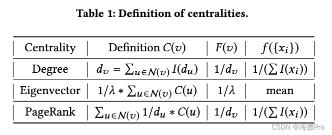
Theorem 3.3. Centrality 、 Centrality of eigenvectors [5]、PageRank Centrality [27] They are the three optimal solutions of our model .

Using lemma 3.4 To prove

lemma 3.4 For any computable function , There is a finite recurrent neural network [24] To calculate it .

It is proved that the process is simple （ Look not to understand ）

---

Theorem 3.5. If node $v$ The centrality of $C(v)$ Satisfy $C(v)={\sum }_{u\in N(u)}F(u)C(u)$ and $F(u)=f(\{F(u),u\in N(v)\})$, among $F$ Is any computable function , that $C(v)$ Is one of the optimal solutions of our model

It is proved that the process is simple （ Look not to understand ）

---

adopt $(F(v),f(\{x_i\}))$ In the table 1 The definition of centrality in , We can easily get degree centrality 、 Centrality of eigenvectors 、PageRank Centrality satisfies theorem 3.5 Conditions , Thus the theorem is completed 3.3 The proof of .

According to the theorem 3.3, For any graph , The methods we proposed are There is such a parameter setting , That is, the learned embeddedness can be one of the three centrality

This proves the expressiveness of our method in capturing different aspects of network structure information related to rule equivalence .

3.6 Analysis and Discussions

In this section , We will introduce out of sample expansion and complexity analysis .

3.6.1 Out-of-sample Extension

For a newly arrived node $v$, If you know its connection to an existing node , We can directly input the embedding of its neighbors into the aggregate function , Usage 1 Get the aggregate representation embedded as the node .

The complexity of this process is $O(d_{v}k)$

• $k$ Is the embedded length ,
• $d_v$ For the node $v$ Degree .

3.6.2 Complexity Analysis

In the process of training , For a single node per iteration $v$, The time complexity of calculating gradient and updating parameters is $O(d_v{k}^2)$

$d_v$ For the node $v$ Degree ,$k$ Is the embedded length

Due to the sampling process ,$d_v$ The degree will not exceed the limit S. Therefore, the overall training complexity is $O(|V|S{k}^{2}I)$

$I$ For the number of iterations

Setting of other parameters

• Embedded length $k$ Usually set to a smaller number , Such as 32,64,128.
• S Set to 300. The number of iterations $I$ Usually very small. , But with the number of nodes $|V|$ irrelevant

therefore , The complexity of the training process and the number of nodes $|V|$ In a linear relationship .

4 EXPERIMENTS

4.1 Baselines and Parameter Settings

Baseline approach

• DeepWalk
• LINE
• node2vec
• struc2vec
• Centralities： Adopt near centrality [26]、 Intermediate centrality [4]、 Centrality of eigenvectors [6] and K-core[17] These four commonly used centrality measures the importance of nodes . Besides , We connect the previous four centrality to one vector as another baseline (Combined)

Parameter setting

For our model , We set up

• Embedded length $k$ by 16
• The weight of the regularizer $\lambda$ by 1
• Finite neighborhood number $S$ by 300

We will be in 4.5 Instructions in section Our model is not very sensitive to these parameters

4.2 Network Visualization

Barbell network visualization

Karate network visualization

4.3 Regular Equivalence Prediction

In this section , We evaluate the learned embeddedness Whether to maintain rule equivalence on two real-world datasets

Data sets

• Jazz[10]
• BlogCatalog [38]

Here we set up two tasks , Include Rule equivalence prediction and Central score prediction

---

For the first mission , We use common similarity measurement methods based on rule equivalence VS[18] As the basic truth value .

The pairwise similarity of two nodes is measured by their embedded inner product .

We sort node pairs according to their similarity , And sort the results with VS. Kendall Sort and compare

Use [1] Rank correlation coefficient To measure the correlation between these two ranks . Its definition is as follows :

The result is shown in Fig. 5 Shown :

---

For the second mission , We take 4.1 The four centrality mentioned in section are calculated as a benchmark

Then hide randomly 20% The node of , Use the remaining nodes to train the linear regression model , Prediction centrality score based on node embedding

After training , We use a regression model to predict the centrality of the shielded nodes

Using the mean square error (Mean Square Error, MSE) Evaluate its performance .MSE The definition is as follows :

among $Y$ Is the observed value ,$\hat{Y}$ For the predicted value .

Because the scales of different centrality have significant differences , We will MSE Value divided by the corresponding average of all node centrality to rescale .

Results such as table 2、 surface 3 Shown .

4.4 Structural Role Classification

In the classification task based on structural role , The label of a node is more associated with its structure information than the label of its adjacent node .

In this section , We evaluate learning embedded in The ability to predict the structural roles of nodes in a given network .

Data sets ： European air traffic network and American air traffic network [29]

Nodes represent airports , The edge indicates the existence of direct navigation .
The total number of people landing and taking off or passing through the airport can be used to measure their activities , Reflect their structural role in the flight network .
By evenly dividing the activity distribution of each airport into one of the four possible tags .

After getting the embedding of the airport , We Training a logical regression prediction based on embedded tags

We randomly selected 10% ~ 90% As training samples , Use the remaining nodes to test performance .

Average accuracy is used to evaluate performance .

The result is shown in Fig. 6 Shown , The solid line represents the network embedding method , The dotted line indicates the central method .

4.5 Parameter Sensitivity

We evaluate the embedding dimension $k$、 Regularizer weights $\lambda$ And the upper bound of neighborhood size $S$ Influence

4.6 Scalability

To prove scalability , We test each epoch Training time for

The result is shown in Fig. 8 Shown

5 CONCLUSION

In this paper , We propose a new depth model to learn the node representation with rule equivalence in the network .

It is assumed that the rule equivalence information of a node has been encoded by the representation of its adjacent nodes , We propose a layer of normalization LSTM Model recursive learning node embedding .

For a given node , The structural importance information of long-distance nodes can be recursively propagated to adjacent nodes , So as to be embedded in its embedding .

therefore , The learned node embedding can reflect the structural information of nodes in a global sense , This is consistent with the equivalence and centrality measures of rules .

The empirical results show that , Our method can significantly and consistently outperform state-of-the-art algorithms .

After reading the summary

The overall idea is generally understood

But because of right LSTM Don't understand

I still don't understand the details

If you need to explore it carefully in the future , Study it carefully ！

Conclusion

The article is only used as a personal study note , Record from 0 To 1 A process of

Hope to help you a little bit , If you have any mistakes, you are welcome to correct them