Reading graph augmentations to learn graph representations (lg2ar)

High quality resource sharing

Learning route guidance （ Click unlock ）	Knowledge orientation	Crowd positioning
🧡 Python Actual wechat ordering applet 🧡	Progressive class	This course is python flask+ Perfect combination of wechat applet , From the deployment of Tencent to the launch of the project , Create a full stack ordering system .
Python Quantitative trading practice	beginner	Take you hand in hand to create an easy to expand 、 More secure 、 More efficient quantitative trading system

Paper information

Paper title ：Learning Graph Augmentations to Learn Graph Representations Author of the paper ：Kaveh Hassani, Amir Hosein Khasahmadi Source of the paper ：2022, arXiv Address of thesis ：download Paper code ：download

1 Introduction

We introduced LG2AR, Learning graph enhancement to learn graph representation , This is an end-to-end automatic graph enhancement framework , Help the encoder learn the generalized representation at the node and graph level .LG2AR It consists of a probability strategy for learning the distribution on the enhancement parameters and a group of probability enhancement heads for learning the distribution on the enhancement parameters . We show that , Compared with previous unsupervised models under linear and semi supervised evaluation protocols ,LG2AR stay 20 Of the graph level and node level benchmarks 18 The most advanced results have been obtained on .

2 Method

The overall framework is as follows ：

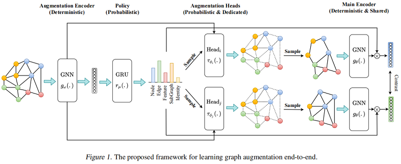
2.1 Augmentation Encoder

Enhanced encoder gω(.):R|V|×dx×R|E|*R|V|×dh×Rdhgω(.):R|V|×dx×R|E|*R|V|×dh×Rdhg_{\omega}(.): \mathbb{R}^{|\mathcal{V}| \times d_{x}} \times \mathbb{R}^{|\mathcal{E}|} \longmapsto \mathbb{R}^{|\mathcal{V}| \times d_{h}} \times \mathbb{R}^{d_{h}} Based on graph GkGkG_{k} Generate node representation  Hv∈R|V|×dhHv∈R|V|×dh\mathbf{H}_{v} \in \mathbb{R}^{|\mathcal{V}| \times d_{h}} And the graph shows   hg∈Rdhhg∈Rdhh_{g} \in \mathbb{R}^{d_{h}} .

Enhanced encoder gω(.)gω(.)g_{\omega}(.) The composition of ：

• • GNN Encoder;
    • Readout function;
    • Two MLP projection head;

2.2 Policy

Policy rμ(.):R|B|×dh*R|τ|rμ(.):R|B|×dh*R|τ|r_{\mu}(.): \mathbb{R}^{|\mathcal{B}| \times d_{h}} \longmapsto \mathbb{R}^{|\tau|} Is a probability module , Receive a batch of graph level representations from the enhancement encoder Hg∈R|B|×dhHg∈R|B|×dh\mathbf{H}_{g} \in \mathbb{R}^{|\mathcal{B}| \times d_{h}} , Construct an enhanced distribution TT\mathcal{T}, Then sample two data enhancements τϕiτϕi\tau_{\phi_{i}} and τϕjτϕj\tau_{\phi_{j}}. Since enhanced sampling over the entire dataset is expensive , In this paper, we choose a small batch processing method to approximate .

Besides ,Policy The order of representations within the batch must remain unchanged , So this paper tries two strategies ：

1. a policy instantiated as a deep set where representations are first projected and then aggregated into a batch representation.
2. a policy instantiated as an RNN where we impose an order on the representations by sorting them based on their L2-norm and then feeding them into a GRU.

This article uses the last hidden state as a batch representation . We observed that GRU The policy is better . The strategy module automates the special trial and error enhancement selection process . To make the gradient flow back to the strategy module , We used a jump connection , And multiply the final graph representation by the enhanced probability of strategy prediction .

2.3 Augmentations

Topological augmentations:

• • node dropping
    • edge perturbation
    • subgraph inducing

Feature augmentation：

• • feature masking

Identity augmentation

Compared with previous work , The enhanced parameters are randomly or heuristically selected , We choose to learn them end-to-end . for example , We are not randomly dropping nodes or calculating the probability proportional to the centrality measure , Instead, a model is trained to predict the distribution of all nodes in the graph , Then samples are taken from it to decide which nodes to discard . And Policy Different modules , Enhancements are conditional on a single graph . We use a dedicated header for each enhancement , Modeled as a two-tier MLP, Learn to enhance the distribution of parameters . The input to the header is the original graph GGG And represent... From the enhancement encoder HvHv\mathbf{H}_{v} and hGhGh_{G}. We use Gumbel-Softmax Technique to sample the learned distribution .

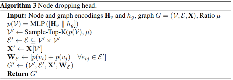
Node Dropping Head

Conditional on node and graph representation , To determine which nodes in the graph to delete .

It receives nodes and graph representations as input , And predict the classification distribution on the nodes . And then use Gumbel-Top-K skill , The distribution is sampled using the ratio superparameter . We also tried Bernoulli sampling , But we observe that it actively reduces nodes in the first few periods , The model cannot be restored in the future . To make the gradient flow back from the augmented graph to the head , We introduce edge weights on augmented graphs , One of the edge weights wijwijw_{i j} Calculated as p(vi)+p(vj)p(vi)+p(vj)p\left(v_{i}\right)+p\left(v_{j}\right), and p(vi)p(vi)p\left(v_{i}\right) Is assigned to the node viviv_{i} Probability .

Algorithm is as follows ：

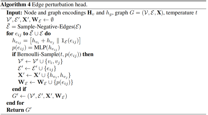
Edge Perturbation Head

Subject to the head and tail nodes , To decide to add / Which edges to delete .

First, random sampling |E||E||\mathcal{E}| Negative edges ( E¯¯¯E¯\overline{\mathcal{E}} ), Form a group of size 2|E|2|E|2|\mathcal{E}| Set of negative and positive edges of E∪E¯¯¯E∪E¯\mathcal{E} \cup \overline{\mathcal{E}}. The edges are represented by [hvi+hvj∥1E(eij)][hvi+hvj‖1E(eij)]\left[h_{v_{i}}+h_{v_{j}} | \mathbb{1}_{\mathcal{E}}\left(e_{i j}\right)\right] ( hvihvih_{v_{i}} and hvjhvjh_{v_{j}} Each represents an edge eijeije_{i j} Representation of the head and tail nodes of ,1E(eij)1E(eij)\mathbb{1}_{\mathcal{E}}\left(e_{i j}\right) Used to judge whether the edge belongs to positivate edge perhaps negative edge ) Input Heads To learn Bernoulli distribution . We use the probability of prediction p(eij)p(eij)p\left(e_{i j}\right) As edge weights , Let the gradient flow back to the head .

Algorithm is as follows ：

Sub-graph Inducing Head
　　 Determine the central node based on the node and graph representation .

It receives nodes and graph representations ( namely [hv∥hg][hv‖hg]\left[h_{v} | h_{g}\right] ) As input , And learn the classification distribution on the nodes . Then the distribution is sampled , Select a central node for each graph , Use with around this node K−hopK−hopK-hop Breadth first search (BFS) Induce a subgraph . We use similar techniques to implement node deletion enhancements , Go back to the original graph by crossing the gradient .

The algorithm process ：

Feature Masking Head
　　 Conditional on node representation , To determine which dimensions of node characteristics to mask . Header receiving node representation hvhvh_v, The Bernoulli distribution is learned on each feature dimension of the original node feature . The distribution is then sampled , Construct a binary mask on the initial feature space mmm. Because the initial node characteristics can be composed of category attributes , So we use a linear layer to project them into a continuous space , To get x′vxv′x_{v}^{\prime}. The augmented graph has the same structure as the original graph , With initial node characteristics x′v⊙mxv′⊙mx_{v}^{\prime} \odot m（⊙⊙\odot Multiply Hadamard ）.

The algorithm process ：

2.4 Base Encoder

Basic encoder gθ(.):R|V′|×d′x×R|V′|×|V′|*R|V′|×dh×Rdhgθ(.):R|V′|×dx′×R|V′|×|V′|*R|V′|×dh×Rdhg_{\theta}(.): \mathbb{R}^{{\left|\mathcal{V}}{\prime}\right| \times d_{x}^{\prime}} \times \mathbb{R}^{{\left|\mathcal{V}}{\prime}\right| \times\left|\mathcal{V}^{\prime}\right|} \longmapsto \mathbb{R}^{{\left|\mathcal{V}}{\prime}\right| \times d_{h}} \times   \mathbb{R}^{d_{h}} Is a shared graph encoder , Enhanced reception enhancement diagram of G′=(V′,E′)G′=(V′,E′)G^{{\prime}=\left(\mathcal{V}}{\prime}, \mathcal{E}^{\prime}\right) Receive an enhancement map from the corresponding enhancement header G′=(V′,E′)G′=(V′,E′)G^{{\prime}=\left(\mathcal{V}}{\prime}, \mathcal{E}^{\prime}\right), And learn a set of node representations H′v∈R|V′|×dhHv′∈R|V′|×dh\mathbf{H}_{v}^{\prime} \in \mathbb{R}^{{\left|\mathcal{V}}{\prime}\right| \times d_{h}} And enhancement diagram G′G′G^{\prime} The figure on shows h′G∈RdhhG′∈Rdhh_{G}^{\prime} \in \mathbb{R}^{d_{h}}. The goal of learning enhancements is to help the base coder learn the invariance of these enhancements , This produces a robust representation . The basic encoder is trained with strategy and enhancement head . In reasoning , The input map is directly input to the base encoder , To calculate the coding of downstream tasks .

2.5 Training

In this paper InfooMax Objective function ：

maxω,μϕi,ϕj,θ1|G|∑G∈G[1|V|∑v∈V[I(hiv,hjG)+I(hjv,hiG)]]maxω,μϕi,ϕj,θ1|G|∑G∈G[1|V|∑v∈V[I(hvi,hGj)+I(hvj,hGi)]]\underset{\omega, \mu \phi_{i}, \phi_{j}, \theta}{\text{max}} \frac{1}{|\mathcal{G}|} \sum\limits _{G \in \mathcal{G}}\left[\frac{1}{|\mathcal{V}|} \sum_{v \in \mathcal{V}}\left[\mathrm{I}\left(h_{v}^{i}, h_{G}^{{j}\right)+\mathrm{I}\left(h_{v}}{j}, h_{G}^{i}\right)\right]\right]

among ,ωω\omega, μμ\mu, ϕiϕi\phi_{i}, ϕjϕj\phi_{j}, θθ\theta Is the parameter of the module to be learned ,hivhvih_{v}^{{i}、hjGhGjh_{G}}{j} Is enhanced by iii and jjj Encoded nodes vvv Sum graph GGG It means ,III Is mutual information estimator . We use Jensen-Shannon MI estimator：

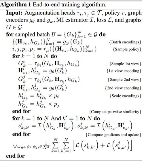
D(.,.):Rdh×Rdh*RD(.,.):Rdh×Rdh*R\mathcal{D}(., .): \mathbb{R}^{d_{h}} \times \mathbb{R}^{d_{h}} \longmapsto \mathbb{R} It's a discriminator , It accepts a node and a graph representation , And score the consistency between them , And realize it as D(hv,hg)=hn⋅hTgD(hv,hg)=hn⋅hgT\mathcal{D}\left(h_{v}, h_{g}\right)=h_{n} \cdot h_{g}^{T}. We provide information from the joint distribution ppp A positive sample of and from the edge p×p_p×pp \times \tilde{p} Negative sample of product , The model parameters are optimized by small batch random gradient descent . We found that , Regularizing the coder by training the random alternation between the base coder and the enhanced coder can help the base coder to generalize better . So , We train our strategy and strengthen our head at every step , But we took samples from Bernoulli , To decide whether to update the base encoder or enhance the weight of the encoder . Algorithm 1 The training process is summarized .

3 Experiments

Data sets

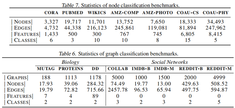
Node classification

Picture classification

4 Conclusion

We introduced LG2AR Compared with the end-to-end framework to automate graph learning . The proposed framework can enhance end-to-end learning 、 View selection policy and encoder , Instead of designing an enhanced ad hoc trial and error process for each data set . Experimental results show that ,LG2AR stay 8 In graph classification 8 The most advanced benchmarking results have been achieved on , Compared with previous unsupervised methods ,7 Node classification benchmark 6 individual . The results also show that ,LG2AR Narrowed the gap with supervision peers . Besides , The results show that , Both learning strategies and learning enhancements help improve performance . In the future work , We plan to study the large-scale pre training and transfer learning ability of the proposed method .

Revise history

2022-06-26  Create articles

Contents of thesis interpretation

• Paper information

• 1 Introduction

• 2 Method

• 2.1 Augmentation Encoder

• 2.2 Policy

• 2.3 Augmentations

• 2.4 Base Encoder

• 2.5 Training

• 3 Experiments

• 4 Conclusion

• Revise history

  __EOF__

  [ Failed to transfer the external chain picture , The origin station may have anti-theft chain mechanism , It is suggested to save the pictures and upload them directly (img-5Xbc9OO9-1656263793313)(https://blog.csdn.net/BlairGrowing)]Blair - Link to this article ：https://blog.csdn.net/BlairGrowing/p/16409040.html

• About bloggers ： Comments and private messages will be answered as soon as possible . perhaps Direct personal trust I .
• Copyright notice ： All articles in this blog except special statement , All adopt BY-NC-SA license agreement . Reprint please indicate the source ！
• Solidarity bloggers ： If you think the article will help you , You can click the bottom right corner of the article **【[ recommend ](javascript:void(0)】** once .