Particle filter PF -- Application in maneuvering target tracking (particle filter vs extended Kalman filter)

Particle filtering PF—— Application in maneuvering target tracking （ Particle filtering VS Extended Kalman filter ）

For the blog tracking code and problem discussion, you can contact ：WX：ZB823618313
For the code and discussion of other tracking and positioning problems, you can also contact

Originality is not easy. , Please give a compliment to all the big guys passing by

One 、 Problem description （ Description of discrete-time nonlinear systems ）

Consider the general nonlinear system model ,
$$\begin{gathered} x_k=f(x_{k-1},w_{k-1}) \\ {z}_k=h(x_k,v_k)\text{\hspace{1em}(1)} \end{gathered}$$
among $x_k$ by $k$ Target state vector at time .$z_k$ by $k$ Time measurement vector （ Sensor data ）. The controller is not considered here $u_k$.$w_k$ and $v_k$ They are process noise sequence and measurement noise sequence , And suppose $w_k$ and $v_k$ Zero mean Gaussian white noise , The variances are $Q_k$ and $R_k$ The Gaussian white noise of , namely $w_k\sim (0,Q_k)$, $v_k\sim (0,R_k)$, And satisfy the following relationship ( Linear Gaussian hypothesis ) by ：
$$\begin{array}{rl}E[w_i{v}_j^{\prime }]& =0\\ E[w_i{w}_j^{\prime }]& =0i\ne j\\ E[v_i{v}_j^{\prime }]& =0i\ne j\end{array}$$

Two 、 Particle filtering PF

The core idea ： Is to use a group of random samples with corresponding weights ( The particle ) To represent the posterior distribution of States . The basic idea of this method is to select an importance probability density and random sampling from it , Get some random samples with corresponding weights , Adjust the weight based on the state observation . And the position of the particles , These samples are then used to approximate the state posterior distribution , Finally, the weighted sum of these samples is taken as the estimated value of the state . Particle filter is not constrained by the linear and Gaussian assumptions of the system model , The state probability density is described in the form of sample rather than function , So that it does not need too many constraints on the probability distribution of state variables , So it is widely used in nonlinear non Gaussian dynamic systems . For all that , At present, the computation of particle filter is still too large 、 Key problems such as particle degradation need to be solved .

Usually, a priori distribution is chosen as the importance density function 、 namely
$$q(x_k|x_{k-1}^{(i)},z_k)=p(x_k|x_{k-1}^{(i)})$$
The importance weight of this function is
$$w_k^{(i)}=w_{k-1}^{(i)}p(z_k|x_k^{(i)})$$
Again $w_k^{(i)}$ Normalization is required to obtain ${\tilde{w}}_k^{(i)}$.

The standard particle filter algorithm steps are ：

Particle filtering PF:
Step 1: according to $p(x_0)$ Sampling to get $N$ A particle $x_0^{(i)}\sim p(x_0)$
For $i=2:N$
  Step 2: The new particle generated from the state transition function is ：$$$x_k^{(i)}\sim p(x_k|x_{k-1}^{(i)})$$
  Step 3: Calculate the importance weight ：$$w_k^{(i)}=w_{k-1}^{(i)}p(z_k|x_k^{(i)})$$
  Step 4: Normalized importance weight ：$${\tilde{w}}_k^{(i)}=\frac{w_k^{(i)}}{{\sum }_{j=1}^N{w}_k^{(j)}}$$
  Step 5: Resample particles using resample method （ Take system resampling as an example ）
  Step 6: obtain $k$ A posteriori state estimation of time ：
$$E[{\hat{x}}_k]=\sum _{i=1}^N{x}_k^{(i)}{\tilde{w}}_k^{(i)}$$
End For

Particle filtering PF Algorithm structure diagram

Algorithm ： System resampling （systematic resampling）
For $i=1:N$
  Step 1: Initialize the cumulative probability density function CDF：$c_1=0$
For $i=2:N$
  Step 2: structure CDF: $c_i=c_{i-1}+w_k^{(i)}$
  Step 3: from CDF Start at the bottom of ：$i=1$
  Step 4: Sampling starting point ：$u_1=\mathcal{U}[0,1/N]$
End For
For $j=1:N$
  Step 5: Along the CDF Move : $u_j=u_1+(j-1)/N$
  Step 6: While $u_j>c_i$
      $i=i+1$
     End While
  Step 7: Assignment particle ：$x_k^{(j)}=x_k^{(i)}$
  Step 8: Assignment weight ：$w_k^{(j)}=1/N$
  Step 9: Assign parent ：$i^{(j)}=i$
End For

3、 ... and 、 Simulation scenario ： 3D radar target tracking

3.1 Simulation scenario （ Three dimensional spiral rising maneuvering target ）

Target model
Consider a three-dimensional uniform turning moving target ：
$$x_{k+1}=F_k{x}_k+G_k{w}_k$$
Where the state vector $x_k=[x_k,{\dot{x}}_k,y_k,{\dot{y}}_k,z_k,{\dot{z}}_k{]}^{\prime }$; The noise is $w_k=[w_x,w_y,w_z{]}^{\prime }$;

The target trajectory is a three-dimensional uniform turning motion model
path of particle ： Spiral rise

If it is a nonlinear target , Then the state transition matrix $F_k$ Replace with Jacobian matrix . In order not to be general, the linear model is used for simulation . It mainly deals with target tracking , The problem of nonlinear filtering in radar measurement .

Radar measurement model
In the three-dimensional case , Radar measurements are range and angle
$$\begin{gathered} r_k^m=r_k+{\tilde{r}}_k \\ {b}_k^m=b_k+{\tilde{b}}_k \\ {e}_k^m=e_k+{\tilde{e}}_k \end{gathered}$$
among
$$\begin{gathered} r_k=\sqrt{(x_k-x_0{)}^{+}(y_k-y_0{)}^2)} \\ {b}_k={\tan }^{-1}\frac{y_k-y_0}{x_k-x_0} \\ {e}_k={\tan }^{-1}\frac{z_k-z_0}{\sqrt{(x_k-x_0{)}^2+(y_k-y_0{)}^2}} \end{gathered}$$
$[x_0,y_0,z_0]$ Is radar coordinates , The general situation is 0. Radar measurement is $z_k=[r_k,b_k,e_k{]}^{\prime }$. The radar measurement variance is
$$R_k=\text{cov}(v_k)=\left[\begin{array}{ccc}{\sigma }_r^2& 0& 0\\ 0& {\sigma }_b^2& 0\\ 0& 0& {\sigma }_e^2\end{array}\right]$$ And ${\sigma }_r=20m$, ${\sigma }_b=20mrad$, ${\sigma }_e=15mrad$.
Performance indicators
RMSE(Root mean-squared error): Montacarlo times $M=500$,${\hat{x}}_{k|k}^i$ For the first time $i$ The estimation obtained from this simulation .
$$\text{RMSE}(\hat{x})=\sqrt{\frac{1}{M}\sum _{i=1}^M({\mathbf{x}}_k-{\hat{\mathbf{x}}}_{k|k}^i)({\mathbf{x}}_k-{\hat{\mathbf{x}}}_{k|k}^i{)}^{\prime }}$$
$$\text{Position RMSE}(\hat{x})=\sqrt{\frac{1}{M}\sum _{i=1}^M(x_k-{\hat{x}}_{k|k}^i{)}^2+(y_k-{\hat{y}}_{k|k}^i{)}^2+(z_k-{\hat{z}}_{k|k}^i{)}^2}$$
$$\text{Velocity RMSE}(\hat{x})=\sqrt{\frac{1}{M}\sum _{i=1}^M({\dot{x}}_k-{\hat{\dot{x}}}_{k|k}^i{)}^2+({\dot{y}}_k-{\hat{\dot{y}}}_{k|k}^i{)}^2+({\dot{z}}_k-{\hat{\dot{z}}}_{k|k}^i{)}^2}$$
ANEES（average normalized estimation error square）,$n$ Is the state dimension ,${\mathbf{P}}_{k|k}^i$ For the first time $i$ The estimated covariance of the output of the secondary simulation filter
$$\text{ANEES}(\hat{x})=\frac{1}{Mn}\sum _{i=1}^M({\mathbf{x}}_k-{\hat{\mathbf{x}}}_{k|k}^i{)}^{\prime }({\mathbf{P}}_{k|k}^i{)}^{-1}({\mathbf{x}}_k-{\hat{\mathbf{x}}}_{k|k}^i)$$

3.2 Track track

3D track ：

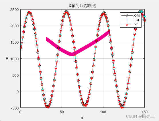
3.3 Tracking error

Four 、 Part of the code

For the blog tracking code and problem discussion, you can contact ：WX：ZB823618313
For the code and discussion of other tracking and positioning problems, you can also contact

Code ： System resampling （systematic resampling）

%%%%%%%%%%%%%%%%%%%%%%%%%%%%%%%%%%%%%%%%%%%%%%%%%%%%%%%%%%%
%  The system reacquires the appearance function 
%  Input parameters ：weight Is the weight corresponding to the original data 
%  Output parameters ：outIndex It's based on weight Filter and copy results 
function outIndex = systematicR(weight);
N=length(weight);
N_children=zeros(1,N);
label=zeros(1,N);
label=1:1:N;
s=1/N;
auxw=0;
auxl=0;
li=0;
T=s*rand(1);
j=1;
Q=0;
i=0;
u=rand(1,N);
while (T<1)
    if (Q>T)
        T=T+s;
        N_children(1,li)=N_children(1,li)+1;
    else
        i=fix((N-j+1)*u(1,j))+j;
        auxw=weight(1,i);
        li=label(1,i);
        Q=Q+auxw;
        weight(1,i)=weight(1,j);
        label(1,i)=label(1,j);
        j=j+1;
    end
end
index=1;
for i=1:N
    if (N_children(1,i)>0)
        for j=index:index+N_children(1,i)-1
            outIndex(j) = i;
        end;
    end;
    index= index+N_children(1,i);
end
%%%%%%%%%%%%%%%%%%%%%%%%%%%%%%%%%%%%%%%%%%%%%%%%%%%%%%%