Ggplot2 color setting summary

Reference resources

http://www.sthda.com/english/wiki/ggplot2-colors-how-to-change-colors-automatically-and-manually

http://www.cookbook-r.com/Graphs/Colors_(ggplot2)/

View colors

col.set.update <- c("#c10023", "#008e17", "#fb8500", "#f60000", "#FE0092", "#bc9000","#4ffc00", "#00bcac", "#0099cc",
                    "#D35400", "#00eefd", "#cf6bd6", "#99cc00", "#aa00ff", "#ff00ff", "#00896e",
                    "#f2a287","#ffb3ff", "#800000", "#77a7b7", "#0053c8", "#00cc99", "#007CC8")
image(1:length(col.set.update),1, as.matrix(1:length(col.set.update)),col=col.set.update,xlab = "", ylab = "")

give the result as follows

prepare data

# Convert dose and cyl columns from numeric to factor variables
ToothGrowth$dose <- as.factor(ToothGrowth$dose)
mtcars$cyl <- as.factor(mtcars$cyl)
head(ToothGrowth)

give the result as follows

head(mtcars)

basic plot

library(ggplot2)
# Box plot
ggplot(ToothGrowth, aes(x=dose, y=len)) +geom_boxplot()
# scatter plot
ggplot(mtcars, aes(x=wt, y=mpg)) + geom_point()

give the result as follows

Color use cases 1

# box plot
ggplot(ToothGrowth, aes(x=dose, y=len)) +
  geom_boxplot(fill='#A4A4A4', color="darkred")
# scatter plot
ggplot(mtcars, aes(x=wt, y=mpg)) + 
  geom_point(color='darkblue')

give the result as follows

Color use cases 2

# Box plot
bp<-ggplot(ToothGrowth, aes(x=dose, y=len, fill=dose)) +
  geom_boxplot()
bp
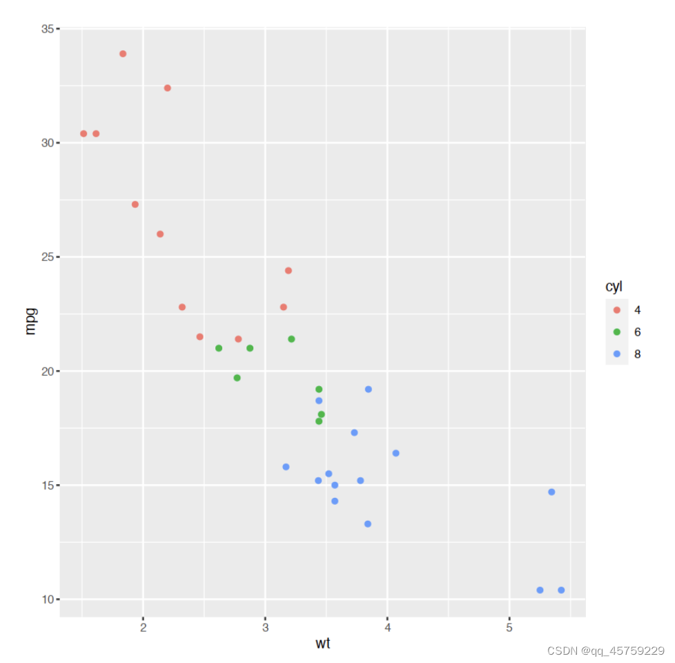
# Scatter plot
sp<-ggplot(mtcars, aes(x=wt, y=mpg, color=cyl)) + geom_point()
sp

give the result as follows

Color use cases 3

# Box plot
bp + scale_fill_hue(l=40, c=35)
# Scatter plot
sp + scale_color_hue(l=40, c=35)

Color use cases 4

# Box plot
bp + scale_fill_manual(values=c("#999999", "#E69F00", "#56B4E9"))
# Scatter plot
sp + scale_color_manual(values=c("#999999", "#E69F00", "#56B4E9"))

give the result as follows

Color use cases 5

# Box plot
bp + scale_fill_manual(breaks = c("2", "1", "0.5"), 
                       values=c("red", "blue", "green"))
# Scatter plot
sp + scale_color_manual(breaks = c("8", "6", "4"),
                        values=c("red", "blue", "green"))

give the result as follows

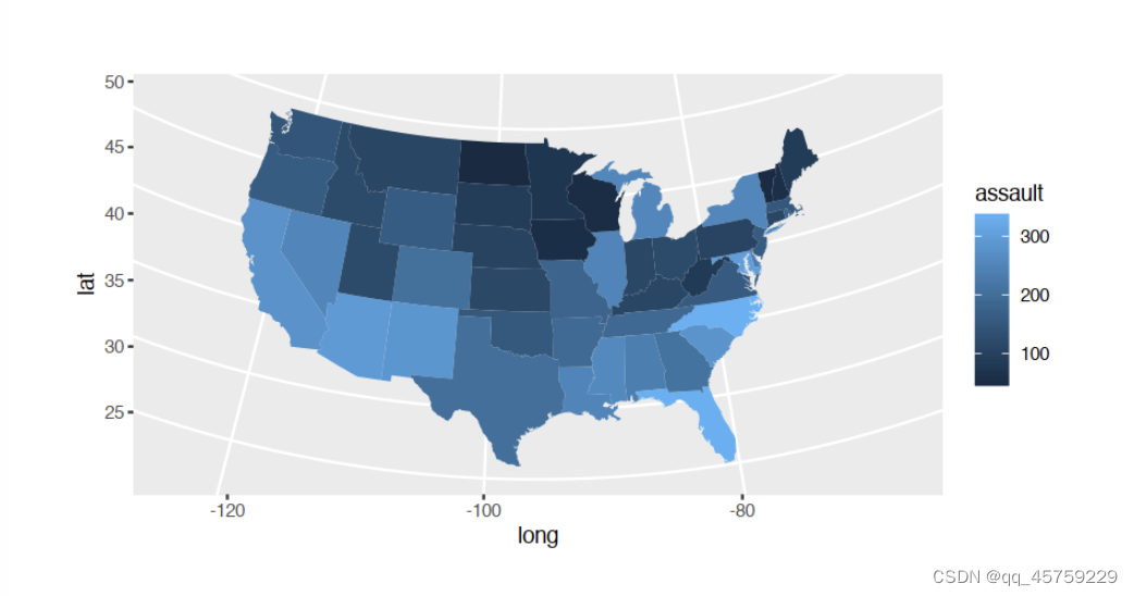
Color use cases 6

library(ggplot2)
if (require("maps")) {
    
states <- map_data("state")
arrests <- USArrests
names(arrests) <- tolower(names(arrests))
arrests$region <- tolower(rownames(USArrests))

choro <- merge(states, arrests, sort = FALSE, by = "region")
choro <- choro[order(choro$order), ]
p=ggplot(choro, aes(long, lat)) +
  geom_polygon(aes(group = group, fill = assault)) +
  coord_map("albers",  lat0 = 45.5, lat1 = 29.5)
print(p)
}

# if (require("maps")) {
    
# p=ggplot(choro, aes(long, lat)) +
# geom_polygon(aes(group = group, fill = assault / murder)) +
# coord_map("albers", lat0 = 45.5, lat1 = 29.5)
# }
# print(p)

Color use cases 7

# Two variables
df <- read.table(header=TRUE, text='
 cond yval
    A 2
    B 2.5
    C 1.6
')

# Three variables
df2 <- read.table(header=TRUE, text='
 cond1 cond2 yval
    A      I 2
    A      J 2.5
    A      K 1.6
    B      I 2.2
    B      J 2.4
    B      K 1.2
    C      I 1.7
    C      J 2.3
    C      K 1.9
')

library(ggplot2)
# Default: dark bars
ggplot(df, aes(x=cond, y=yval)) + geom_bar(stat="identity")
# Bars with red outlines
ggplot(df, aes(x=cond, y=yval)) + geom_bar(stat="identity", colour="#FF9999") 
# Red fill, black outlines
ggplot(df, aes(x=cond, y=yval)) + geom_bar(stat="identity", fill="#FF9999", colour="black")


# Standard black lines and points
ggplot(df, aes(x=cond, y=yval)) + 
    geom_line(aes(group=1)) +     # Group all points; otherwise no line will show
    geom_point(size=3)
# Dark blue lines, red dots
ggplot(df, aes(x=cond, y=yval)) + 
    geom_line(aes(group=1), colour="#000099") +  # Blue lines
    geom_point(size=3, colour="#CC0000")         # Red dots

give the result as follows

Color use cases 8

# Box plot
bp + scale_fill_brewer(palette="Dark2")
# Scatter plot
sp + scale_color_brewer(palette="Dark2")

give the result as follows

Color use cases 9

# Install
#install.packages("wesanderson")
# Load
library(wesanderson)
# Box plot
bp+scale_fill_manual(values=wes_palette(n=3, name="Royal1"))
# Scatter plot
sp+scale_color_manual(values=wes_palette(n=3, name="Royal1"))

give the result as follows

Color use cases 10

# Box plot
bp + scale_fill_grey() + theme_classic()
# Scatter plot
sp + scale_color_grey() + theme_classic()

give the result as follows

Color use cases 11

# Box plot
bp + scale_fill_grey(start=0.8, end=0.2) + theme_classic()
# Scatter plot
sp + scale_color_grey(start=0.8, end=0.2) + theme_classic()

Color use cases 12

# Color by qsec values
sp2<-ggplot(mtcars, aes(x=wt, y=mpg, color=qsec)) + geom_point()
sp2
# Change the low and high colors
# Sequential color scheme
sp2+scale_color_gradient(low="blue", high="red")
# Diverging color scheme
mid<-mean(mtcars$qsec)
sp2+scale_color_gradient2(midpoint=mid, low="blue", mid="white",
                     high="red", space ="Lab" )

give the result as follows

Color use cases 13

set.seed(1234)
x <- rnorm(200)
# Histogram
hp<-qplot(x =x, fill=..count.., geom="histogram") 
hp
# Sequential color scheme
hp+scale_fill_gradient(low="blue", high="red")

Color use cases 14

# Scatter plot
# Color points by the mpg variable
sp3<-ggplot(mtcars, aes(x=wt, y=mpg, color=mpg)) + geom_point()
sp3
# Gradient between n colors
sp3+scale_color_gradientn(colours = rainbow(5))

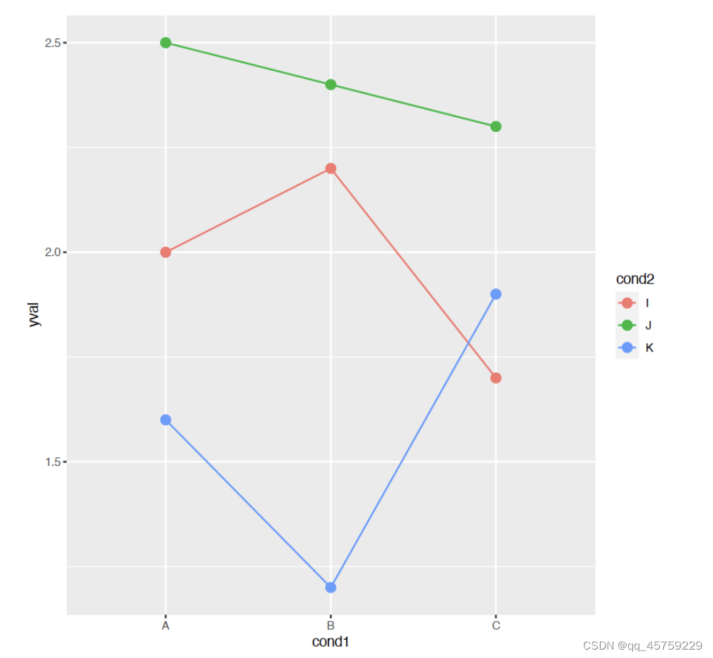
Color use cases 15

# Bars: x and fill both depend on cond2
ggplot(df, aes(x=cond, y=yval, fill=cond)) + geom_bar(stat="identity")

# Bars with other dataset; fill depends on cond2
ggplot(df2, aes(x=cond1, y=yval)) + 
    geom_bar(aes(fill=cond2),   # fill depends on cond2
             stat="identity",
             colour="black",    # Black outline for all
             position=position_dodge()) # Put bars side-by-side instead of stacked

# Lines and points; colour depends on cond2
ggplot(df2, aes(x=cond1, y=yval)) + 
    geom_line(aes(colour=cond2, group=cond2)) + # colour, group both depend on cond2
    geom_point(aes(colour=cond2),               # colour depends on cond2
               size=3)                          # larger points, different shape
## Equivalent to above; but move "colour=cond2" into the global aes() mapping
# ggplot(df2, aes(x=cond1, y=yval, colour=cond2)) + 
# geom_line(aes(group=cond2)) +
# geom_point(size=3)