Natural language inference with attention and fine tuning Bert pytorch

One 、 Natural language inference and data sets

When it comes to deciding whether one sentence can be inferred from another , Or it is necessary to eliminate redundancy between sentences by identifying semantically equivalent sentences , It is not enough to know how to classify a text sequence . contrary , We need to be able to infer pairs of text sequences .

1. Natural language inference

Natural language inference （natural language inference） Main research hypothesis （hypothesis） Can I go from Premise （premise） Infer from , Both of them are text sequences . In other words , Natural language inference determines the logical relationship between a pair of text sequences . There are usually three types of relationships ：

• implication (entailment): The hypothesis can be inferred from the previous proposition .
• contradiction (contradiction): The negation of the hypothesis can be inferred from the antecedent .
• Neutral (neutral): All the other things .

Natural language inference is also known as the task of identifying text implication .

2. Stanford natural language inference dataset

Stanford natural language inference corpus （Stanford Natural Language Inference,SNLI By 500000 A collection of English sentence pairs with labels . Intensive training includes 550000 Yes , The test intensity is 10000 Yes , Three tags in training set and test set “ implication ”、“ contradiction ” and “ Neutral ” It's balanced. .

import os
import re
import torch
from torch import nn
from d2l import torch as d2l

#@save
d2l.DATA_HUB['SNLI'] = (
    'https://nlp.stanford.edu/projects/snli/snli_1.0.zip',
    '9fcde07509c7e87ec61c640c1b2753d9041758e4')

data_dir = d2l.download_extract('SNLI')

def read_snli(data_dir, is_train):
    """ take SNLI Data set parsing is the premise 、 Assumptions and labels """
    def extract_text(s):
        #  Delete parentheses 
        s = re.sub('\\(', '', s)
        s = re.sub('\\)', '', s)
        #  Two or more consecutive spaces leave only one space 
        s = re.sub('\\s{2,}', ' ', s)
        return s.strip()
    #  implication :0, contradiction :1, Neutral :2
    label_set = {
    'entailment': 0, 'contradiction': 1, 'neutral': 2}
    file_name = os.path.join(data_dir, 'snli_1.0_train.txt'
                             if is_train else 'snli_1.0_test.txt')
    with open(file_name, 'r') as f:
        rows = [row.split('\t') for row in f.readlines()[1:]]
    premises = [extract_text(row[1]) for row in rows if row[0] in label_set]
    hypotheses = [extract_text(row[2]) for row in rows if row[0] in label_set]
    labels = [label_set[row[0]] for row in rows if row[0] in label_set]
    return premises, hypotheses, labels

• Load data set

class SNLIDataset(torch.utils.data.Dataset):
    """ Used for loading SNLI Custom datasets for datasets """
    def __init__(self, dataset, num_steps, vocab=None):
        self.num_steps = num_steps
        all_premise_tokens = d2l.tokenize(dataset[0])
        all_hypothesis_tokens = d2l.tokenize(dataset[1])
        if vocab is None:
            self.vocab = d2l.Vocab(all_premise_tokens + \
                all_hypothesis_tokens, min_freq=5, reserved_tokens=['<pad>'])
        else:
            self.vocab = vocab
        self.premises = self._pad(all_premise_tokens)
        self.hypotheses = self._pad(all_hypothesis_tokens)
        self.labels = torch.tensor(dataset[2])
        print('read ' + str(len(self.premises)) + ' examples')

    def _pad(self, lines):
        return torch.tensor([d2l.truncate_pad(
            self.vocab[line], self.num_steps, self.vocab['<pad>'])
                         for line in lines])

    def __getitem__(self, idx):
        return (self.premises[idx], self.hypotheses[idx]), self.labels[idx]

    def __len__(self):
        return len(self.premises)

call read_snli Functions and SNLIDataset Class to download SNLI Data sets , And return the results of training set and test set DataLoader example , And the vocabulary of the training set . Be careful , The vocabulary constructed from the training set must be used as the vocabulary of the test set . therefore , The model trained in the training set will not know any new lexical elements from the test set .

def load_data_snli(batch_size, num_steps=50):
    """ download SNLI Data sets and returns data iterators and vocabularies """
    data_dir = d2l.download_extract('SNLI')
    train_data = read_snli(data_dir, True)
    test_data = read_snli(data_dir, False)
    train_set = SNLIDataset(train_data, num_steps)
    test_set = SNLIDataset(test_data, num_steps, train_set.vocab)
    train_iter = torch.utils.data.DataLoader(train_set, batch_size,
                                             shuffle=True)
    test_iter = torch.utils.data.DataLoader(test_set, batch_size,
                                            shuffle=False)
    return train_iter, test_iter, train_set.vocab

Two 、 Using attention to infer natural language

1. Model

Compared with preserving the order of lexical elements in premises and assumptions , We can align the word elements in one text sequence with each word element in another text sequence , Then compare and aggregate this information , To predict the logical relationship between premises and assumptions . It is similar to the lexical alignment between source and target sentences in machinetranslation , The lexical alignment between presuppositions and hypotheses can be accomplished flexibly through the attention mechanism .

---

• Be careful

The first step is to align the word elements in one text sequence with each word element in another sequence . Alignment is done using weighted averaging “ soft ” alignment , Where, ideally, the larger weight is associated with the lexical element to be aligned .

Soft alignment using attention mechanisms ：$\mathbf{A}=({\mathbf{a}}_1,\dots ,{\mathbf{a}}_m)$ and $\mathbf{B}=({\mathbf{b}}_1,\dots ,{\mathbf{b}}_n)$ Indicates premises and assumptions , The number of lexical elements is $m$ and $n$, among ${\mathbf{a}}_i,{\mathbf{b}}_j\in {\mathbb{R}}^d$. For soft alignment , Attention weight $e_{ij}\in \mathbb{R}$ The calculation for the ：
$$e_{ij}=f({\mathbf{a}}_i{)}^{\top }f({\mathbf{b}}_j)$$
The function $f$ It's below mlp Multi layer perceptron defined in function . The output dimension consists of mlp Of num_hiddens Parameter assignment .

def mlp(num_inputs, num_hiddens, flatten):
    net = []
    net.append(nn.Dropout(0.2))
    net.append(nn.Linear(num_inputs, num_hiddens))
    net.append(nn.ReLU())
    if flatten:
        net.append(nn.Flatten(start_dim=1))
    net.append(nn.Dropout(0.2))
    net.append(nn.Linear(num_hiddens, num_hiddens))
    net.append(nn.ReLU())
    if flatten:
        net.append(nn.Flatten(start_dim=1))
    return nn.Sequential(*net)

In the upper form ,$f$ Input separately ${\mathbf{a}}_i$ and ${\mathbf{b}}_j$, Instead of putting them together in pairs as input . This decomposition technique leads to $f$ Only $m+n$ Calculation per time （ Linear complexity ）, instead of $mn$ Time calculation （ Quadratic complexity ）. Normalize the attention weight , Calculate the weighted average of all lexical vectors in the hypothesis , To get a hypothetical representation , The assumptions and premises are indexed $i$ For soft alignment ：
$${\mathbf{\beta }}_i=\sum _{j=1}^n\frac{\exp (e_{ij})}{{\sum }_{k=1}^n\exp (e_{ik})}{\mathbf{b}}_j.$$

Again , The index in the calculation assumption is $j$ The soft alignment of each lexical element of and the premise lexical element ：

$${\mathbf{\alpha }}_j=\sum _{i=1}^m\frac{\exp (e_{ij})}{{\sum }_{k=1}^m\exp (e_{kj})}{\mathbf{a}}_i.$$

Definition Attend Class to calculate assumptions （beta） And input premises A Soft alignment and premise （alpha） And input assumptions B Soft alignment .

class Attend(nn.Module):
    def __init__(self, num_inputs, num_hiddens, **kwargs):
        super(Attend, self).__init__(**kwargs)
        self.f = mlp(num_inputs, num_hiddens, flatten=False)

    def forward(self, A, B):
        # A/B The shape of the ：（ Batch size , Sequence A/B The number of lexical elements ,embed_size）
        # f_A/f_B The shape of the ：（ Batch size , Sequence A/B The number of lexical elements ,num_hiddens）
        f_A = self.f(A)
        f_B = self.f(B)
        # e The shape of the ：（ Batch size , Sequence A The number of lexical elements , Sequence B The number of lexical elements ）
        e = torch.bmm(f_A, f_B.permute(0, 2, 1))
        # beta The shape of the ：（ Batch size , Sequence A The number of lexical elements ,embed_size）,
        #  It means sequence B Is soft aligned to the sequence A Every word element of (beta Of the 1 Dimensions )
        beta = torch.bmm(F.softmax(e, dim=-1), B)
        # alpha The shape of the ：（ Batch size , Sequence B The number of lexical elements ,embed_size）,
        #  It means sequence A Is soft aligned to the sequence B Every word element of (alpha Of the 1 Dimensions )
        alpha = torch.bmm(F.softmax(e.permute(0, 2, 1), dim=-1), A)
        return beta, alpha

• Compare

Next , Compare a lexical element in a sequence with another sequence in which the lexical element is soft aligned . Be careful , In soft alignment , All morphemes in a sequence （ Although they may have different attention weights ） Compare with the lexical elements in another sequence . for example , Aforementioned “ Be careful ” Step determine... In the premise “need” and “sleep” Are consistent with the hypothetical “tired” alignment , Will be right “ tired - Need sleep ” Compare .

In the comparison step , A join of words from one sequence and aligned words from another sequence are fed into a function $g$（ A multi-layer sensor ）：

$$\begin{gathered} {\mathbf{v}}_{A,i}=g([{\mathbf{a}}_i,{\mathbf{\beta }}_i]),i=1,\dots ,m \\ {\mathbf{v}}_{B,j}=g([{\mathbf{b}}_j,{\mathbf{\alpha }}_j]),j=1,\dots ,n \end{gathered}$$
among ,${\mathbf{v}}_{A,i}$ Refer to , All the lexical elements in the hypothesis and the lexical elements in the premise $i$ Soft alignment , Then with the word yuan $i$ Comparison ;${\mathbf{v}}_{B,j}$ Refer to , The lexical elements in all premises and the lexical elements in hypotheses $i$ Soft alignment , Then with the word yuan $i$ Comparison .

Below Compare Classes define comparison steps .

class Compare(nn.Module):
    def __init__(self, num_inputs, num_hiddens, **kwargs):
        super(Compare, self).__init__(**kwargs)
        self.g = mlp(num_inputs, num_hiddens, flatten=False)

    def forward(self, A, B, beta, alpha):
        V_A = self.g(torch.cat([A, beta], dim=2))
        V_B = self.g(torch.cat([B, alpha], dim=2))
        return V_A, V_B

• polymerization

There are two sets of comparison vectors ${\mathbf{v}}_{A,i}$（$i=1,\dots ,m$） and ${\mathbf{v}}_{B,j}$（$j=1,\dots ,n$）, This information will be aggregated to infer logical relationships . First, sum the two sets of comparison vectors ：

$${\mathbf{v}}_A=\sum _{i=1}^m{\mathbf{v}}_{A,i},{\mathbf{v}}_B=\sum _{j=1}^n{\mathbf{v}}_{B,j}.$$

Next , Provide a link between the two summation results to the function $h$（ A multi-layer sensor ）, To obtain the classification results of logical relations ：

$$\hat{\mathbf{y}}=h([{\mathbf{v}}_A,{\mathbf{v}}_B]).$$

The aggregation steps are as follows Aggregate Definition in class .

class Aggregate(nn.Module):
    def __init__(self, num_inputs, num_hiddens, num_outputs, **kwargs):
        super(Aggregate, self).__init__(**kwargs)
        self.h = mlp(num_inputs, num_hiddens, flatten=True)
        self.linear = nn.Linear(num_hiddens, num_outputs)

    def forward(self, V_A, V_B):
        #  Sum the two sets of comparison vectors respectively 
        V_A = V_A.sum(dim=1)
        V_B = V_B.sum(dim=1)
        #  Link the two summation results to the multi-layer perceptron 
        Y_hat = self.linear(self.h(torch.cat([V_A, V_B], dim=1)))
        return Y_hat

• Integrate code

By paying attention to step 、 The comparison step and the aggregation step are combined , Define a decomposable attention model to jointly train these three steps .

class DecomposableAttention(nn.Module):
    def __init__(self, vocab, embed_size, num_hiddens, num_inputs_attend = 100,
                 num_inputs_compare = 200, num_inputs_agg = 400, **kwargs):
        super(DecomposableAttention, self).__init__(**kwargs)
        self.embedding = nn.Embedding(len(vocab), embed_size)
        self.attend = Attend(num_inputs_attend, num_hiddens)
        self.compare = Compare(num_inputs_compare, num_hiddens)
        #  Yes 3 Two possible outputs ： implication 、 Contradiction and neutrality 
        self.aggregate = Aggregate(num_inputs_agg, num_hiddens, num_outputs=3)

    def forward(self, X):
        premises, hypotheses = X
        A = self.embedding(premises)
        B = self.embedding(hypotheses)
        beta, alpha = self.attend(A, B)
        V_A, V_B = self.compare(A, B, beta, alpha)
        Y_hat = self.aggregate(V_A, V_B)
        return Y_hat

2. Training and evaluation models

#  Reading data sets 
batch_size, num_steps = 256, 50
train_iter, test_iter, vocab = d2l.load_data_snli(batch_size, num_steps)

#  Creating models 
embed_size, num_hiddens, devices = 100, 200, d2l.try_all_gpus()
net = DecomposableAttention(vocab, embed_size, num_hiddens)
glove_embedding = d2l.TokenEmbedding('glove.6b.100d')
embeds = glove_embedding[vocab.idx_to_token]
net.embedding.weight.data.copy_(embeds)

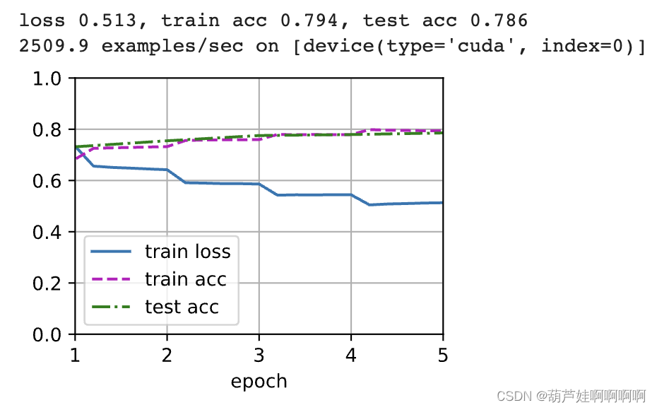
#  Training and evaluation models 
lr, num_epochs = 0.001, 4
trainer = torch.optim.Adam(net.parameters(), lr=lr)
loss = nn.CrossEntropyLoss(reduction="none")
d2l.train_ch13(net, train_iter, test_iter, loss, trainer, num_epochs,
    devices)

If an error , Change it matplotlib Version of !pip install matplotlib==‘3.0’

3. forecast

def predict_snli(net, vocab, premise, hypothesis):
    """ The logical relationship between prediction premises and assumptions """
    net.eval()
    premise = torch.tensor(vocab[premise], device=d2l.try_gpu())
    hypothesis = torch.tensor(vocab[hypothesis], device=d2l.try_gpu())
    label = torch.argmax(net([premise.reshape((1, -1)),
                           hypothesis.reshape((1, -1))]), dim=1)
    return 'entailment' if label == 0 else 'contradiction' if label == 1 \
            else 'neutral'
predict_snli(net, vocab, ['he', 'is', 'good', '.'], ['he', 'is', 'bad', '.'])
# contradiction

3、 ... and 、 fine-tuning BERT Make natural language inferences

stay BERT This blog uses a smaller data set WikiText-2 Pre training BERT（ The original BERT The model is pre trained on a larger corpus ）. Here are two versions of the pre training BERT：“bert.base” With the original BERT As big as the base model , It requires a lot of computing resources to fine tune ,“bert.small” It's a small version .

1. Load pre-trained BERT

import json
import multiprocessing
import os
import torch
from torch import nn
from d2l import torch as d2l

d2l.DATA_HUB['bert.base'] = (d2l.DATA_URL + 'bert.base.torch.zip',
                             '225d66f04cae318b841a13d32af3acc165f253ac')
d2l.DATA_HUB['bert.small'] = (d2l.DATA_URL + 'bert.small.torch.zip',
                              'c72329e68a732bef0452e4b96a1c341c8910f81f')

Two pre trained BERT Each model contains a that defines a vocabulary “vocab.json” File and a pre training parameter “pretrained.params” file .load_pretrained_model function Load pre trained BERT Parameters .

def load_pretrained_model(pretrained_model, num_hiddens, ffn_num_hiddens,
                          num_heads, num_layers, dropout, max_len, devices):
    data_dir = d2l.download_extract(pretrained_model)
    #  Define an empty vocabulary to load a predefined vocabulary 
    vocab = d2l.Vocab()
    vocab.idx_to_token = json.load(open(os.path.join(data_dir,'vocab.json')))
    vocab.token_to_idx = {
    token: idx 
                         for idx, token in enumerate(vocab.idx_to_token)}
    bert = d2l.BERTModel(len(vocab), num_hiddens, norm_shape=[256],
                         ffn_num_input=256, ffn_num_hiddens=ffn_num_hiddens,
                         num_heads=4, num_layers=2, dropout=0.2,
                         max_len=max_len, key_size=256, query_size=256,
                         value_size=256, hid_in_features=256,
                         mlm_in_features=256, nsp_in_features=256)
    #  Load pre training BERT Parameters 
    bert.load_state_dict(torch.load(os.path.join(
                                    data_dir, 'pretrained.params')))
    return bert, vocab

2. For fine tuning BERT Data set of

about SNLI The downstream task of the dataset is natural language inference , Defines a dataset class SNLIBERTDataset. In each sample , Premises and assumptions form a pair of text sequences , And packaged into a BERT Input sequence . The fragment index is used to distinguish BERT Input the premises and assumptions in the sequence . Use predefined BERT The maximum length of the input sequence （max_len）, Continue to remove the last mark of the longer text in the input text pair , Until you meet max_len.

class SNLIBERTDataset(torch.utils.data.Dataset):
    def __init__(self, dataset, max_len, vocab=None):
        all_premise_hypothesis_tokens = [[
            p_tokens, h_tokens] for p_tokens, h_tokens in zip(
            *[d2l.tokenize([s.lower() for s in sentences])
              for sentences in dataset[:2]])]

        self.labels = torch.tensor(dataset[2])
        self.vocab = vocab
        self.max_len = max_len
        (self.all_token_ids, self.all_segments,
         self.valid_lens) = self._preprocess(all_premise_hypothesis_tokens)
        print('read ' + str(len(self.all_token_ids)) + ' examples')

    def _preprocess(self, all_premise_hypothesis_tokens):
        pool = multiprocessing.Pool(4)  #  Use 4 A process 
        out = pool.map(self._mp_worker, all_premise_hypothesis_tokens)
        all_token_ids = [token_ids for token_ids, segments, valid_len in out]
        all_segments = [segments for token_ids, segments, valid_len in out]
        valid_lens = [valid_len for token_ids, segments, valid_len in out]
        return (torch.tensor(all_token_ids, dtype=torch.long),
                torch.tensor(all_segments, dtype=torch.long),
                torch.tensor(valid_lens))

    def _mp_worker(self, premise_hypothesis_tokens):
        p_tokens, h_tokens = premise_hypothesis_tokens
        self._truncate_pair_of_tokens(p_tokens, h_tokens)
        tokens, segments = d2l.get_tokens_and_segments(p_tokens, h_tokens)
        token_ids = self.vocab[tokens] + [self.vocab['<pad>']] \
                             * (self.max_len - len(tokens))
        segments = segments + [0] * (self.max_len - len(segments))
        valid_len = len(tokens)
        return token_ids, segments, valid_len

    def _truncate_pair_of_tokens(self, p_tokens, h_tokens):
        #  by BERT In input '<CLS>'、'<SEP>' and '<SEP>' The word element retains its position 
        while len(p_tokens) + len(h_tokens) > self.max_len - 3:
            if len(p_tokens) > len(h_tokens):
                p_tokens.pop()
            else:
                h_tokens.pop()

    def __getitem__(self, idx):
        return (self.all_token_ids[idx], self.all_segments[idx],
                self.valid_lens[idx]), self.labels[idx]

    def __len__(self):
        return len(self.all_token_ids)

Download the SNLI After the dataset , Instantiation SNLIBERTDataset Class to generate training and test samples . These samples will be read in small batches during the training and testing of natural language inference .

devices = d2l.try_all_gpus()
bert, vocab = load_pretrained_model(
    'bert.small', num_hiddens=256, ffn_num_hiddens=512, num_heads=4,
    num_layers=2, dropout=0.1, max_len=512, devices=devices)
#  If there is an out of memory error , Please reduce “batch_size”. In the original BERT In the model ,max_len=512
batch_size, max_len, num_workers = 512, 128, d2l.get_dataloader_workers()
data_dir = d2l.download_extract('SNLI')
train_set = SNLIBERTDataset(d2l.read_snli(data_dir, True), max_len, vocab)
test_set = SNLIBERTDataset(d2l.read_snli(data_dir, False), max_len, vocab)
train_iter = torch.utils.data.DataLoader(train_set, batch_size, shuffle=True,
                                   num_workers=num_workers)
test_iter = torch.utils.data.DataLoader(test_set, batch_size,
                                  num_workers=num_workers)

3. fine-tuning BERT

Fine tuning for natural language inference BERT Only an additional multi-layer perceptron is required , The multi-layer perceptron consists of two fully connected layers . This multi-layer perceptron will be special “<cls>” Morpheme Of BERT Indicates that a transformation has been made , This lexical element encodes the information of premise and hypothesis at the same time ( Three outputs for natural language inference )： implication 、 Contradiction and neutrality .

class BERTClassifier(nn.Module):
    def __init__(self, bert):
        super(BERTClassifier, self).__init__()
        self.encoder = bert.encoder
        self.hidden = bert.hidden
        self.output = nn.Linear(256, 3)

    def forward(self, inputs):
        tokens_X, segments_X, valid_lens_x = inputs
        encoded_X = self.encoder(tokens_X, segments_X, valid_lens_x)
        return self.output(self.hidden(encoded_X[:, 0, :]))

stay BERT in ,MaskLM Classes and NextSentencePred Class has some parameters in the multi-layer perceptron it uses , These parameters are pre training BERT Part of the model parameters , These parameters are only used to calculate the masking language model loss and the next sentence prediction loss in the pre training process . These two loss functions are independent of fine tuning downstream applications , So when BERT Fine tuning ,MaskLM and NextSentencePred The parameters of the multi-layer perceptron used in... Will not be updated .

In order to allow parameters with old gradients , sign ignore_stale_grad=True stay step function d2l.train_batch_ch13 Is set to . Using this function SNLI Training set of （train_iter） And test set （test_iter） Yes net Model for training and evaluation .

(Colab use GPU Ran close to 20 minute )

net = BERTClassifier(bert)
lr, num_epochs = 1e-4, 5
trainer = torch.optim.Adam(net.parameters(), lr=lr)
loss = nn.CrossEntropyLoss(reduction='none')
d2l.train_ch13(net, train_iter, test_iter, loss, trainer, num_epochs,
    devices)