Task03 probability theory

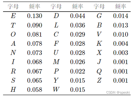
（1） Frequency table in English writing

Random phenomena and probability

Probability theory mainly studies random phenomena that can be repeated in large numbers ‘

（1） Randomized trials ： Repeatable random phenomenon is also called random experiment
（2） Sample points ： All possible basic results
（3） sample space ： All basic results of random phenomena （ Sample points ） Is called the sample space of this random phenomenon
（4） Random events ： The set of some basic results of random phenomena is called random events
（5） The relationship between events ：

• contain
• equal
• Not compatible with each other
• Inevitable and impossible events
  （6） Operation of events ：
• Opposition
• and
• hand over
• Bad
  （7） Axiomatic definition of probability ：
• Nonnegative axiom
• Regularity axiom
• Additivity axiom
  （8） Independence of events

Analog frequency approximation probability

import numpy as np
import pandas as pd
import matplotlib.pyplot as plt
%matplotlib inline
# Provided with  MATLAB  Similar drawings  API
# call matplotlib.pyplot The graph function of plot() When drawing , Or generate a figure When it comes to canvases , It can be directly in your python console There's an image inside .
plt.style.use("ggplot")
#  Canvas style   Use plt.style.available You can find a style suitable for graphics 
import warnings
warnings.filterwarnings("ignore")
# Ignore the red warning in the code 
plt.rcParams['font.sans-serif']=['SimHei','Songti SC','STFangsong']
# Define the drawing default properties   Set the font 
plt.rcParams['axes.unicode_minus']=False
# Used to display negative sign normally 
import seaborn as sns

import random
def Simulate_coin(test_num):
random_seed(100)# Define random number seed 
coin_list=[1 if random.random()>=0.5]else 0 for i range(test_num)]# Simulation test results 
# Greater than or equal to 0.5 Of course 1  Otherwise 0
coin_frequence = np.cumsum(coin_list)/（np.arrange(len(coin_list))+1）
# The front of the calculation is 1 Probability 
plt.figure(figsize=(10,6))
# mapping , Specify the size of the canvas 
plt.plot(np.arrange(len(coin_list))+1,coin_frequence,c='blue',alpha=0.7)
# Number of abscissa tests , Ordinate frequency 
plt.xlabel("test_index")
plt.ylabel("frequence")
plt.title(str(test_num)+" times")
plt.show()
Simulate_coin(test_num = 600)
Simulate_coin(test_num = 1000)
Simulate_coin(test_num = 6000)
Simulate_coin(test_num = 10000)

Conditional probability , The multiplication formula , Full probability formula and Bayesian formula

（1） Conditional probability
$$P(A\mid B)=\frac{P(AB)}{P(B)}$$
（2） The multiplication formula

• if $P(B)>0$, be $P(AB)=P(B)P(A\mid B)$
• if $P\left(A_1{A}_2\cdots A_{n-1}\right)>0$, be $P\left(A_1{A}_2\cdots A_n\right)=P\left(A_1\right)P\left(A_2\mid A_1\right)P\left(A_3\mid A_1{A}_2\right)\cdots P\left(A_n\mid A_1{A}_2\cdots A_{n-1}\right)$

exp:

$$P\left({\bar{A}}_1{\bar{A}}_2{A}_3\right)=P\left({\bar{A}}_1\right)$$

$$P\left({\bar{A}}_2\mid {\bar{A}}_1\right)P\left(A_3\mid {\bar{A}}_1{\bar{A}}_2\right)=\frac{90}{100}\cdot \frac{89}{99}\cdot \frac{10}{98}=0.0826.$$

(3) All probability formula
$$P(A)=\sum _{i=1}^{n}P\left(A\mid B_i\right)P\left(B_i\right)$$

（4） Bayes' formula

With simple $P\left(A\mid B_k\right)$ Solve complex problems $P\left(B_k\mid A\right)$

$$P\left(B_k\mid A\right)=\frac{P(A{B}_k)}{P(A)}$$

The numerator and denominator are expanded by multiplication formula and full probability formula respectively , namely ：
$$P\left(B_k\mid A\right)=\frac{P\left(A\mid B_k\right)P\left(B_k\right)}{{\sum }_{i=1}^{n}P\left(A\mid B_i\right)P\left(B_i\right)},k=1,2,\cdots ,n$$

Three questions

Contestants will see three closed doors , There is a car behind one of them , You can win the car by selecting the door that has the car behind you , And behind each of the other two doors 1 A goat . When the contestants selected a door , But not to turn it on , The host will open one of the remaining two doors , Expose it 1 A goat . The host will then ask the contestants if they want to change another door that is still closed . The problem is ： Whether changing another door will increase the chances of competitors winning the car ？
When the host doesn't open the door , The probability of winning the car is $1/3$
$$\begin{array}{rl}& P(A)=P(B)=P(C)=1/3\end{array}$$
hypothesis ：
A: The contestant chooses the second door , The first door is the car ,
B: The contestant chooses the second door , The second door is the car ,
C: The contestant chooses the second door , The third door is the car ,
D: The host opens the first door
According to the semantics, we can list the probability formula
$$\begin{array}{r}P(D|A)=0P(D|B)=1/2P(D|C)=1\end{array}$$
$$\begin{array}{rl}& \text{According to the Bayes formula ：}\\ & P(D)=P(A)P(D\mid A)+P(B)P(D\mid B)+P(C)P(D\mid C)=1/2\\ & P(C\mid D)=P(C)P(D\mid C)/P(D)=2/3\\ & P(B\mid D)=P(B)P(D\mid B)/P(D)=1/3\end{array}$$

import random
class MontyHall:
  def __init__(self,n): # Constructors 
	self.n=n# Number of tests 
	self.change=0# Record how many times you have to change to get the car 
	sellf.No_change=0# No change 
  def start(self):
	for i in range(self,n):
		door_list=[1,2,3]# Three doors 
		challenger_door = random.choice(door_list)
		## One of them was chosen at random 
		car_door=  random.choice(door_list)
		# Car door 
		## The remaining doors not selected by the Challenger 
		door_list.remove(challenger_door)
		
		if challenger_door==car_door:
			host_door = random.choice(door_list)
			door.remove(host_door)
		# You can only take the car without changing it 
			self.No_change+=1
		else:
			self.change+=1
		# I can't get the car until I change it 
		  print(" The probability of changing and getting the car ：%.2f " % (self.change/self.n * 100) + "%")
        print(" The probability of getting the car without changing it ：%.2f"% (self.No_change/self.n * 100) + "%")
		
if __name__ == "__main__":
    mh = MontyHall(1000000)
    mh.start()  

One dimensional random variables

Random variables are divided into discrete and continuous
There are two ways to calculate the probability of a random event represented by a random variable ： Direct calculation （ Use the distribution function to calculate ） and Indirect calculation method （ Use the density function to calculate ）

$$F(x)=P(X⩽x)$$

$$0⩽F(x)⩽1$$

• $F(-\infty )={\lim }_{x\to -\infty }F(x)=0$ , This is because of the incident “ $X⩽-\infty$ " It's an impossible event .
• $F(+\infty )={\lim }_{x\to +\infty }F(x)=1$, This is because of the incident “ $X⩽+\infty$ " It's an inevitable event .

$$\begin{array}{rl}& P(a<X⩽b)=F(b)-F(a)\\ & P(X=a)=F(a)-F(a-0)\\ & P(X⩾b)=1-F(b-0)\\ & P(X>b)=1-F(b)\\ & P(X<b)=F(b-0)\\ & P(a<X<b)=F(b-0)-F(a)\\ & P(a⩽X⩽b)=F(b)-F(a-0)\\ & P(a⩽X<b)=F(b-0)-F(a-0)\end{array}$$

$a$ And $b$ When continuous , Yes
$$F(a-0)=F(a),F(b-0)=F(b)$$

Use density function to calculate the probability in a certain area

$$P(a⩽X⩽b)={\int }_a^{b}p(x)dx$$

discrete :
Distribution column

$$\begin{array}{cccccc}X& x_1& x_2& \cdots & x_n& \cdots \\ P& p\left(x_1\right)& p\left(x_2\right)& \cdots & p\left(x_n\right)& \cdots \end{array}$$

Continuous type ：
exp:
The density function of Cauchy distribution , Take the derivative of the distribution function

##  Given the density function of Cauchy distribution, find the distribution function 
from sympy import *
x = symbols('x')
p_x = 1/pi*(1/(1+x**2))
integrate(p_x,(x,-∞,x))
# integral   From negative infinity to x

from sympy import *
x = symbols('x')
f_x = 1/pi*(atan(x)+pi/2)
diff(f_x,x,1)
# Derivation 

Uniform distribution ：

The density function is
$U(a,b)$
$$p(x)=\{\begin{array}{ll}\frac{1}{b-a},& a⩽x⩽b\\ 0,& \text{ Other }\end{array}$$

The distribution function is ：
$$F(x)=\{\begin{array}{ll}0,& x<a\\ \frac{x-a}{b-a},& a⩽x<b\\ 1,& x⩾b\end{array}$$

exp:

a = float(0)
b = float(1)
#numpy.linspace() The function is used to generate a sequence of numbers in a linear space in uniform steps 
x = np.linspace(a,b)
y = np.full(shape=len(x),fill_value=1/(b-a))
#np.full Construct an array 
plt.plot(x,y,"b",linewidth=2)
plt.ylim(0,1,2)
plt.xlim(-1,2)
plt.xlabel('X')
plt.ylabel('p(x)')
plt.title('uniform distribution')
plt.show()

An index distribution

$$p(x)=\{\begin{array}{rl}\lambda e^{-\lambda x},& x⩾0\\ 0,& x<0\end{array}$$
$$F(x)=\{\begin{array}{ll}1-{\mathrm{e}}^{-\lambda x},& x⩾0\\ 0,& x<0\end{array}$$

lam = float(1.5)
x = np.linspace(0,15,100)
y = lam*np.e**(-lam*x)

plt.plot(x,y,"b",linewidth=2)
plt.xlim(-5,10)
plt.xlabel('X')
plt.ylabel('p(x)')
plt.title(' An index distribution ')
plt.show()

Gaussian distribution

from sympy import *
from sympy.abc import mu,sigma
x = symbols('X')
p_x = 1/(sqer(2*pi)*sigma)*E**(-(x-mu)**2/(2*sigma**2))
integrate(p_x,(x,-∞,x))

import math
mu = float(0)
mul = float(2)
sigma1 = float(1)
sigma2 = float(1.25)*float(1.25)
sigma3 = float(0.25)
x = np.linspace(-5, 5, 1000)
y1 = np.exp(-(x - mu)**2 / (2 * sigma1**2)) / (math.sqrt(2 * math.pi) * sigma1)
y2 = np.exp(-(x - mu)**2 / (2 * sigma2**2)) / (math.sqrt(2 * math.pi) * sigma2)
y3 = np.exp(-(x - mu)**2 / (2 * sigma3**2)) / (math.sqrt(2 * math.pi) * sigma3)
y4 = np.exp(-(x - mu1)**2 / (2 * sigma1**2)) / (math.sqrt(2 * math.pi) * sigma1)
plt.plot(x,y1,"b",linewidth=2,label=r'$\mu=0,\sigma=1$') 
plt.plot(x,y2,"orange",linewidth=2,label=r'$\mu=0,\sigma=1.25$') 
plt.plot(x,y3,"yellow",linewidth=2,label=r'$\mu=0,\sigma=0.5$') 
plt.plot(x,y4,"b",linewidth=2,label=r'$\mu=2,\sigma=1$',ls='--') 
plt.axvline(x=mu,ls='--')
plt.text(x=0.05,y=0.5,s=r'$\mu=0$')
plt.axvline(x=mu1,ls='--')
plt.text(x=2.05,y=0.5,s=r'$\mu=2$')
plt.xlim(-5,5)
plt.xlabel('X')
plt.ylabel('p (x)')
plt.title('normal distribution')
plt.legend()
plt.show()

change mu

change σ

Exponential distribution calculation

from scipy.stats import expon # An index distribution 
x = np.linspace(0.01,10,1000)
plt.plot(x,expon.pdf(x),'r-',lw=5,alpha=0.6,label='expon pdf')
 # pdf Means to find the value of density function 
 # cdf Means to find the value of the distribution function 
plt.xlabel("X")
plt.ylabel("p (x)")
plt.legend()
#plt.legend Create Legend 
plt.show()

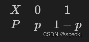
(1)0-1 Distribution

(2) The binomial distribution

(3) Poisson distribution

Poisson distribution calculation

#  Contrast different lambda Influence on Poisson distribution 
import math
#  Construct the calculation function of Poisson distribution column 
def poisson(lmd,x):
    return pow(lmd,x)/math.factorial(x)*math.exp(-lmd)
x = [i+1 for i in range(10)]
# Define Poisson distribution Columns 
lmd1 = 0.8
lmd2 = 2.0
lmd3 = 4.0
lmd4 = 6.0

p_lmd1 = [poisson(lmd1,i) for i in x]
p_lmd2 = [poisson(lmd2,i) for i in x]
p_lmd3 = [poisson(lmd3,i) for i in x]
p_lmd4 = [poisson(lmd4,i) for i in x]

plt.scatter(np.array(x), p_lmd1, c='b',alpha=0.7)
plt.axvline(x=lmd1,ls='--')
plt.text(x=lmd1+0.1,y=0.1,s=r"$\lambda=0.8$")
plt.ylim(-0.1,1)
plt.xlabel("X")
plt.ylabel("p (x)")
plt.title(r"$\lambda = 0.8$")
plt.show()

plt.scatter(np.array(x), p_lmd2, c='b',alpha=0.7)
plt.axvline(x=lmd2,ls='--')
plt.text(x=lmd2+0.1,y=0.1,s=r"$\lambda=2.0$")
plt.ylim(-0.1,1)
plt.xlabel("X")
plt.ylabel("p (x)")
plt.title(r"$\lambda = 2.0$")
plt.show()

plt.scatter(np.array(x), p_lmd3, c='b',alpha=0.7)

plt.axvline(x=lmd3,ls='--')
plt.text(x=lmd3+0.1,y=0.1,s=r"$\lambda=4.0$")
plt.ylim(-0.1,1)
plt.xlabel("X")
plt.ylabel("p (x)")
plt.title(r"$\lambda = 4.0$")
plt.show()

plt.scatter(np.array(x), p_lmd4, c='b',alpha=0.7)
plt.axvline(x=lmd4,ls='--')
plt.text(x=lmd4+0.1,y=0.1,s=r"$\lambda=6.0$")
plt.ylim(-0.1,1)
plt.xlabel("X")
plt.ylabel("p (x)")
plt.title(r"$\lambda = 6.0$")
plt.show()

plt.scatter Scatter plot
axvline The function draws a vertical line across the entire subgraph
ylim Set or query y Axis range

from scipy.stats import binom
#scipy.stats In bag binom Class objects represent binomial distributions .
n = 10
p = 0.5
x = np.arange(1,n+1,1)
pList = binom.pmf(x,n,p)
#stats.binom.pmf(X,n,p)  For the probability density 
plt.plot(x,pList,marker='o',alpha = 0.7,linestyle = 'None')

plt.vlines(x, 0, pList)
# Drawing data sets 
plt.xlabel(' A random variable ： Flip a coin 10 Time ')
plt.ylabel(' probability ')
plt.title(' The binomial distribution ：n=%d,p=%0.2f' % (n,p))
plt.show()

Numerical characteristics of one-dimensional random variables ： expect 、 variance 、 Quantile and median

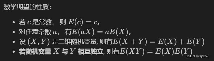
（1） Mathematical expectation
The number of positional features of the distribution
Discrete random variable ：

Continuous random variables ：
If the integral is finite ：

---

exp:

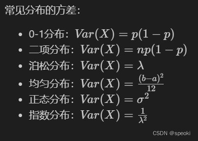
(2) Standard deviation and variance
Reflect the fluctuation of random variables

variance

discrete ：

Continuous type ：


Standard deviation

scipy Calculate the mean and variance of common distributions

#  Use scipy Calculate the mean and variance of common distributions ：( If you forget the formula, look it up directly , There is no need to look up books )
from scipy.stats import bernoulli   # 0-1 Distribution 
from scipy.stats import binom   #  The binomial distribution 
from scipy.stats import poisson  #  Poisson distribution 
from scipy.stats import rv_discrete #  Custom discrete random variables 
from scipy.stats import uniform #  Uniform distribution 
from scipy.stats import expon #  An index distribution 
from scipy.stats import norm #  Normal distribution 
from scipy.stats import rv_continuous  #  Custom continuous random variables 

print("0-1 The numerical characteristics of the distribution ： mean value :{}; variance :{}; Standard deviation :{}".format(bernoulli(p=0.5).mean(), 
                                  bernoulli(p=0.5).var(), 
                                  bernoulli(p=0.5).std()))
print(" The binomial distribution b(100,0.5) The digital characteristics of ： mean value :{}; variance :{}; Standard deviation :{}".format(binom(n=100,p=0.5).mean(), 
                                  binom(n=100,p=0.5).var(), 
                                  binom(n=100,p=0.5).std()))
##  Simulate the specific distribution of the dice 
xk = np.arange(6)+1
pk = np.array([1.0/6]*6)
print(" Poisson distribution P(0.6) The digital characteristics of ： mean value :{}; variance :{}; Standard deviation :{}".format(poisson(0.6).mean(), 
                                  poisson(0.6).var(), 
                                  poisson(0.6).std()))
print(" The numerical characteristics of a particular discrete random variable ： mean value :{}; variance :{}; Standard deviation :{}".format(rv_discrete(name='dice', values=(xk, pk)).mean(), 
                                  rv_discrete(name='dice', values=(xk, pk)).var(), 
                                  rv_discrete(name='dice', values=(xk, pk)).std()))
print(" Uniform distribution U(1,1+5) The digital characteristics of ： mean value :{}; variance :{}; Standard deviation :{}".format(uniform(loc=1,scale=5).mean(), 
                                  uniform(loc=1,scale=5).var(), 
                                  uniform(loc=1,scale=5).std()))
print(" Normal distribution N(0,0.0001) The digital characteristics of ： mean value :{}; variance :{}; Standard deviation :{}".format(norm(loc=0,scale=0.01).mean(), 
                                  norm(loc=0,scale=0.01).var(), 
                                  norm(loc=0,scale=0.01).std()))

lmd = 5.0  #  Exponentially distributed lambda = 5.0
print(" An index distribution Exp(5) The digital characteristics of ： mean value :{}; variance :{}; Standard deviation :{}".format(expon(scale=1.0/lmd).mean(), 
                                  expon(scale=1.0/lmd).var(), 
                                  expon(scale=1.0/lmd).std()))

##  Custom standard normal distribution 
class gaussian_gen(rv_continuous):
    def _pdf(self, x): # tongguo 
        return np.exp(-x**2 / 2.) / np.sqrt(2.0 * np.pi)
gaussian = gaussian_gen(name='gaussian')
print(" Numerical characteristics of standard normal distribution ： mean value :{}; variance :{}; Standard deviation :{}".format(gaussian().mean(), 
                                  gaussian().var(), 
                                  gaussian().std()))

##  Custom exponential distribution 
import math
class Exp_gen(rv_continuous):
    def _pdf(self, x,lmd):
        y=0
        if x>0:
            y = lmd * math.e**(-lmd*x)
        return y
Exp = Exp_gen(name='Exp(5.0)')
print("Exp(5.0) The numerical characteristics of the distribution ： mean value :{}; variance :{}; Standard deviation :{}".format(Exp(5.0).mean(), 
                                  Exp(5.0).var(), 
                                  Exp(5.0).std()))

##  Customize the distribution through the distribution function 
class Distance_circle(rv_continuous):                 # Custom distribution xdist
    """  The radial direction is r Throw a little in the circle of , Random variable of distance from point to center of circle X The distribution function of is : if x<0: F(x) = 0; if 0<=x<=r: F(x) = x^2 / r^2 if x>r: F(x)=1 """
    def _cdf(self, x, r):                   # The cumulative distribution function defines the random variable 
        f=np.zeros(x.size)                  # The function value is initialized to 0
        index=np.where((x>=0)&(x<=r))           #0<=x<=r
        f[index]=((x[index])/r[index])**2       #0<=x<=r
        index=np.where(x>r)                     #x>r
        f[index]=1                              #x>r
        return f
dist = Distance_circle(name="distance_circle")
print("dist The numerical characteristics of the distribution ： mean value :{}; variance :{}; Standard deviation :{}".format(dist(5.0).mean(), 
                                  dist(5.0).var(), 
                                  dist(5.0).std()))

（3） Quantile and median
The cumulative probability is equal to p The corresponding random variable value x by p quantile
$$F\left(x_p\right)={\int }_{-\infty }^{x_p}p(x)\mathrm{d}x=p$$

Upper and lower side mutual conversion conversion formula
$$x_p^{\prime }=x_{1-p},x_p=x_{1-p}^{\prime }$$
The median is P=0.5 The quantile of hour
$$F\left(x_{0.5}\right)={\int }_{-\infty }^{x_{0.5}}p(x)\mathrm{d}x=0.5$$

Median and mean can comprehensively explain the distribution of data
The mean is affected by extreme data

Use python Calculate the standard normal distribution 0.25,0.5（ Median ）,0.75,0.95 Quantile .

from scipy.stats import norm
print(" Standard normal distribution 0.25 quantile ：",norm(loc=0,scale=1).ppf(0.25))   #  Use ppf Calculate quantile point 
print(" Standard normal distribution 0.5 quantile ：",norm(loc=0,scale=1).ppf(0.5))
print(" Standard normal distribution 0.75 quantile ：",norm(loc=0,scale=1).ppf(0.75))
print(" Standard normal distribution 0.95 quantile ：",norm(loc=0,scale=1).ppf(0.95))

Multidimensional random variables and their joint distributions 、 Marginal distribution 、 Conditional distribution

（1）n Dimensional random variable

（1.1）n Joint distribution function of dimensional random variables

（1.2）n Joint density function of dimensional random variables

（1.3） Multidimensional discrete random variable joint distribution column

#  Draw the joint probability density surface of two-dimensional normal distribution 
from scipy.stats import multivariate_normal
from mpl_toolkits.mplot3d import axes3d
# mpl_toolkits.mplot3d A tool kit for drawing three-dimensional drawings 
x, y = np.mgrid[-5:5:.01, -5:5:.01]  #  Return to multidimensional structure 
#mgrid usage ： Return to multidimensional structure 
pos = np.dstack((x, y))
# since  x and  y It's all two-dimensional ,np.dstack By inserting a size of  1  To extend them 
rv = multivariate_normal([0.5, -0.2], [[2.0, 0.3], [0.3, 0.5]])
# multivariate_normal Random sampling from multivariate normal distribution   Function of 
z = rv.pdf(pos)
# pdf Find the value of the density function 
plt.figure('Surface', facecolor='lightgray',figsize=(12,8))
ax = plt.axes(projection='3d')
ax.set_xlabel('X', fontsize=14)
ax.set_ylabel('Y', fontsize=14)
ax.set_zlabel('P (X,Y)', fontsize=14)
ax.plot_surface(x, y, z, rstride=50, cstride=50, cmap='jet')
plt.show()

#  Draw the joint probability density contour map of two-dimensional normal distribution 
from scipy.stats import multivariate_normal
x, y = np.mgrid[-1:1:.01, -1:1:.01]
pos = np.dstack((x, y))
rv = multivariate_normal([0.5, -0.2], [[2.0, 0.3], [0.3, 0.5]])
z = rv.pdf(pos)
fig = plt.figure(figsize=(8,6))
ax2 = fig.add_subplot(111)
ax2.set_xlabel('X', fontsize=14)
ax2.set_ylabel('Y', fontsize=14)
ax2.contourf(x, y, z, rstride=50, cstride=50, cmap='jet')
plt.show()

（2.1） Marginal distribution function ：
$$\underset{y\to \infty }{\lim }F(x,y)=P(X⩽x,Y<\infty )=P(X⩽x),$$

（2.2） Marginal density function

$$\begin{array}{rl}& F_X(x)=F(x,\infty )={\int }_{-\infty }^x\left({\int }_{-\infty }^{\infty }p(u,v)\mathrm{d}v\right)\mathrm{d}u={\int }_{-\infty }^x{p}_X(u)\mathrm{d}u\\ & F_Y(y)=F(\infty ,y)={\int }_{-\infty }^y\left({\int }_{-\infty }^{\infty }p(u,v)\mathrm{d}u\right)\mathrm{d}v={\int }_{-\infty }^y{p}_Y(v)\mathrm{d}v\end{array}$$

#  Find the marginal density function  p_{X}(x)
from sympy import *
x = symbols('x')
y = symbols('y')
p_xy = Piecewise((1,And(x>0,x<1,y<x,y>-x)),(0,True))
integrate(p_xy, (y, -oo, oo))   ##  because 0<x<1 When , that x>-x, namely 2x

#  Find the marginal density function  p_{Y}(y)
integrate(p_xy, (x, -oo, oo))   ##  because |y|<x,0<x<1 when , therefore y It must be (-1,1)

（2.3） Marginal distribution column
x Marginal distribution column of
$$\sum _{j=1}^{\infty }P\left(X=x_i,Y=y_j\right)=P\left(X=x_i\right),i=1,2,\cdots$$

y Marginal distribution column of .
$$\sum _{i=1}^{\infty }P\left(X=x_i,Y=y_j\right)=P\left(Y=y_j\right),j=1,2,\cdots$$
(3) Conditional distribution

#  Find the density function  p_{Y}(y)
from sympy import *
from sympy.abc import lamda,m,p,k
x = symbols('x')
y = symbols('y')
f_p = lamda**m/factorial(m)*E**(-lamda)*factorial(m)/(factorial(k)*factorial(m-k))*p**k*(1-p)**(m-k)
summation(f_p, (m, k, +oo))

（3.1） Full probability formula and Bayes formula for continuous cases

Numerical characteristics of multidimensional random variables ： Expectation vector 、 Covariance and covariance matrix 、 Correlation coefficient and correlation coefficient matrix 、 Conditional expectation

(1) Expectation vector
$n$ The dimensional random vector is $\mathbf{X}={\left(X_1,X_2,\cdots ,X_n\right)}^{\prime }$ There are mathematical expectations for each component

Mathematical expectation vector （ It is generally a column vector ）

$$E(\mathbf{X})={\left(E\left(X_1\right),E\left(X_2\right),\cdots ,E\left(X_n\right)\right)}^{\prime }$$
（2） Covariance and covariance matrix ：
（2.1） covariance ：
$$\mathrm{Cov}(X,Y)=E[(X-E(X))(Y-E(Y))]$$
$$\mathrm{Cov}(X,Y)=E(XY)-E(X)E(Y)$$

When $\mathrm{Cov}(X,Y)>0$ when , call $X$ And $Y$ positive correlation

When $\mathrm{Cov}(X,Y)<0$ when , call $X$ And $Y$ negative correlation

When $\mathrm{Cov}(X,Y)=0$ when , call $X$ And $Y$ Unrelated

If random variable $X$ And $Y$ Are independent of each other , be $\mathrm{Cov}(X,Y)=0$
$$\mathrm{Cov}(X,Y)=\mathrm{Cov}(Y,X).$$
$$\mathrm{Cov}(X,a)=0$$
$$\mathrm{Cov}(aX,bY)=ab\mathrm{Cov}(X,Y).$$
$$\mathrm{Cov}(X+Y,Z)=\mathrm{Cov}(X,Z)+\mathrm{Cov}(Y,Z)$$

For any two-dimensional random variable $(X,Y)$, Yes
$$\mathrm{Var}(X\pm Y)=\mathrm{Var}(X)+\mathrm{Var}(Y)\pm 2\mathrm{Cov}(X,Y)$$

exp:
$$p(x,y)=\{\begin{array}{ll}3x,& 0<y<x<1,\\ 0,& \text{ other . }\end{array}$$
seek $\mathrm{Cov}(X,Y)$.

#  Find the covariance 
from sympy import *
from sympy.abc import lamda,m,p,k
x = symbols('x')
y = symbols('y')
p_xy = Piecewise((3*x,And(y>0,y<x,x<1)),(0,True))
E_xy = integrate(x*y*p_xy, (x, -oo, oo),(y,-oo,oo))
E_x = integrate(x*p_xy, (x, -oo, oo),(y,-oo,oo))
E_y = integrate(y*p_xy, (x, -oo, oo),(y,-oo,oo))
E_xy - E_x*E_y