Mathematical modeling -- integer programming

Catalog

Basic concepts

Integer programming model solution

Integer linear programming model

Monte Carlo solution  

Genetic algorithm  

  other

---

Basic concepts

The programming problem in which some or all of the decision variables must be rounded off is called Integer programming .

Pure integer programming ： All decision variables are integers ; mixed integer programming ： Some of the decision variables are integer values , The other part is not an integer ;0-1 Integer programming ： The decision variable can only take 0 or 1 Integer programming of .

Integer linear programming model （ Some or all decision variables in a linear programming model are integers ） General form ：

Sometimes , Or by introducing 0-1 Variables linearize some specific nonlinear constraints . If there is m Two mutually exclusive constraints , That is, only one condition can work at a time , Then introduce m individual 0-1 Variable ：

And a sufficiently large normal number M, Then the following group m+1 The three constraints meet the above requirements ：

Integer programming model solution

Integer linear programming model

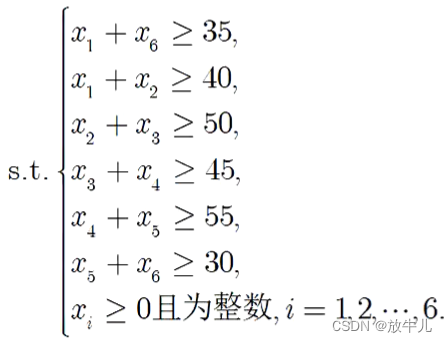
For example, solve the following integer programming ：

clc,clear
prob = optimproblem;
x = optimvar('x',6,'Type','integer','LowerBound',0);
prob.Objective = sum(x);
con = optimconstr(6); % Create an empty optimization constraint array 
a = [35,40,50,45,55,30];
con(1) = x(1)+x(6) >= 35;
for i = 1:5
    con(i+1) = x(i)+x(i+1) >= a(i+1);
end
prob.Constraints.con = con;
[sol,fval,flag] = solve(prob);
sol.x,fval

ans =

    35
     5
    45
     0
    55
     0
fval =

   140

  You can also make it up like this ：

Monte Carlo solution  

Monte Carlo method is also called computer simulation method , It is similar to being in a square area with a known area , Find the area of the irregular figure surrounded by it , Sprinkle a large number of beans , According to the number of beans , Find the area .

unifrnd(A,B)% Generated by A and B Specify the upper and lower endpoints [A,B] A continuous and uniformly distributed random array R.

R = unifrnd(A,B,m,n,...)

R = unifrnd(A,B,[m,n,...])% return m*n*... Array

rng(1)%1 As a random number seed , For consistency comparison .

rng('shuffle')% Provide seeds for the random number generator based on the current time .

tic% Timing begins

toc% End of the timing

B = all(A)% If A It's two-dimensional , The number of columns is n, be B For one 1*n Matrix . If A The elements of a column in are all true , be B The corresponding element in is 1. If A It's three-dimensional , be B Columns of 、 Number of pages and A identical ,B The number of lines is 1. The case that is higher than three dimensions can be analogized .

For example, solving nonlinear integer programming ：x All are integers

clc,clear
rng(0);
p0 = 0;
n = 10^6;
tic;
for i = 1:n
    x = randi([0,99],1,5);
    [f,g] = mente(x);
    if all(g <= 0)
        if p0 <f
            x0 = x;p0 = f;
        end
    end
end
x0,p0,toc

function [f,g] = mente(x)
f = x(1)^2+x(2)^2+3*x(3)^2+4*x(4)^2+2*x(5)^2-8*x(1)-2*x(2)...
    -3*x(3)-x(4)-2*x(5);
g = [sum(x)-400
    x(1)+2*x(2)+2*x(3)+x(4)+6*x(5)-800
    2*x(1)+x(2)+6*x(3)-200
    x(3)+x(4)+5*x(5)-200];
end

x0 =

    46    98     1    99     3
p0 =

       50273

after 0.927967 second .

Genetic algorithm  

 fun It's the objective function （ Only the minimum value ）,nvars Represents the number of variables ,A、b Linear inequality constraint ,Aeq、beq Linear equal sign constraint ,lb、ub Represents upper and lower bounds ,nonlcon Represents a nonlinear constraint ,intcon Indicate which variables are integer variables ,options Used to indicate other optimization settings .

Also use the example above ：

clc,clear
f = @(x) x(1)^2+x(2)^2+3*x(3)^2+4*x(4)^2+2*x(5)^2-8*x(1)-2*x(2)...
    -3*x(3)-x(4)-2*x(5);
A = [1,1,1,1,1;
    1,2,2,1,6;
    2,1,6,0,0;
    0,0,1,1,5];
b = [400;800;200;200];
[x,fvdisc] = ga(@(x)-f(x),5,A,b,[],[],zeros(1,5),99*ones(1,5),[],[1:5])

 @(x)-f(x) Indicates that another anonymous function is defined -f(x)

x =

    50    99     0    99    20
fvdisc =

      -51568 

  other

The process of solving practical problems is ： Problem analysis 、 The model assumes 、 Symbol description 、 model .

MATLAB The middle line is too long to use "..." To wrap