Using keras and LSTM to realize time series prediction of long-term trend memory -lstnet

Hello everyone , Long time no see . I finally finished my thesis and defense .
Today, let's realize the multi-dimensional time series prediction of long-term trend
At the same time, it will provide a complete prediction process and relevant evaluation indicators , Used to evaluate the accuracy of prediction .
The algorithm comes from a classic paper LSTNet, See LSTNet Detailed explanation - You know
Open source code from LSTNet_keras , The data set is replaced and simplified .’
LSTNet It is a model specially established for multivariable time series prediction , In traffic flow , Experiments were carried out on the data of power consumption and exchange rate , Good results . Published in 2018 Year of ACM SIGIR The meeting .

---

Data is introduced

This data set is a pollution data set , We need to use the multidimensional time series to predict pollution This dimension , use 80% As a training set ,20% As test set .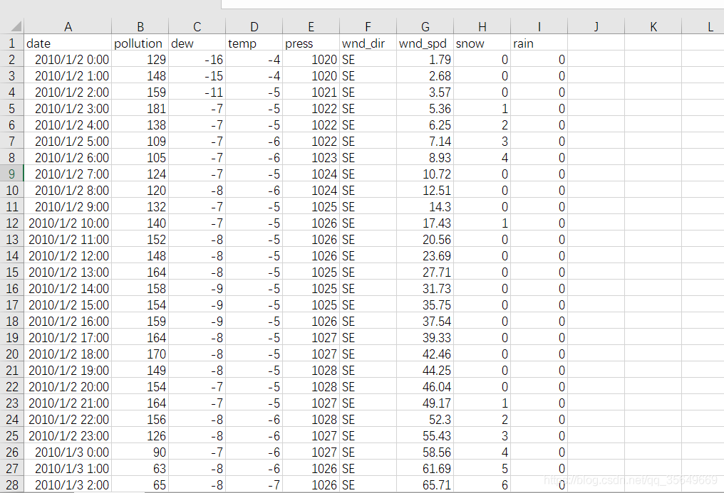

pollution Data trends are as follows :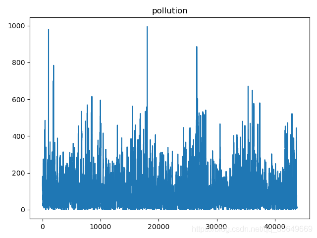

Model is introduced

LSTNet The network structure of is shown in the figure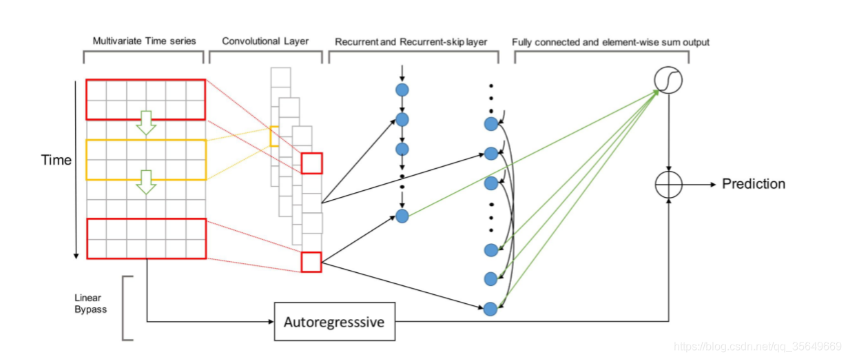

We can see that a convolution layer is used Two layer recurrent neural network ( Used in the paper RNN or GRU, In this article, I used LSTM), As you can see, on the second layer of the graph, an implementation called " Skip layer " Structure , Used to realize the memory of very long-term trends . But in fact, it is data transformation rather than LSTM Structural changes .

For skipping layers , For example, input data [1,2,3,4,5,6,7,8,9,10,11,12], A series of data transformations will be carried out to
[[1,7] , [2,8] , [3,9] , [4,10] , [5,11] , [6,12]], And then type in LSTM In , Realize the memory of long-term trends . Then integrate two layers LSTM Result , Input into the full connection layer .

about Autogressive, It uses the autoregressive mechanism of full connection layer simulation , It will intercept the data of several time steps , Input to the mechanism of the full connection layer . Get the results . It is called in the paper " Linear components are added to the model ", In fact, it has a good effect in predicting some peaks .

Model implementation

For the original model The implementation of the second skip layer requires a large number of data slices , It will be very time consuming
But this article refers to LSTNet_keras Decompose the input into (1) Short term time series , Such as (t-3, t-2, t-1, t) and (2) Long jump time series , Such as (t-2xskip, t-skip, t). The result is as good as the original , But much faster .

Data structure

The data structure adopts the following code , See the end of the article for specific usage github Source code

def create_dataset(dataset, look_back,skip):
    '''  Process the data  '''
    dataX,dataX2,dataY = [],[],[]
    #len(dataset)-1  unnecessary   But some situations can be avoided bug
    for i in range(look_back*skip,len(dataset)-1):
        dataX.append(dataset[(i-look_back):i,:])
        dataY.append(dataset[i, :])
        temp=[]
        for j in range(i-look_back*skip,i,skip):
            temp.append(dataset[j,:])
        dataX2.append(temp)

    TrainX = np.array(dataX)
    TrainX2 = np.array(dataX2)
    TrainY = np.array(dataY)
    return TrainX, TrainX2 , TrainY

The model code

For the initial LSTNet for , Only a single one-dimensional convolution is used to process the data , Then carry out data transformation . But for this simplified version , Data transformation is carried out when constructing data . So we need two one-dimensional convolutions , Then they were given the same weight .
In the model z refer to AR Model implementation

def LSTNet(trainX1,trainX2,trainY,config):

    input1 = Input(shape=(trainX1.shape[1], trainX1.shape[2]))
    conv1 = Conv1D(filters=48, kernel_size=6, strides=1, activation='relu')  # for input1
    # It's a probelm that I can't find any way to use the same Conv1D layer to train the two inputs,
    conv2 = Conv1D(filters=48, kernel_size=6 , strides=1, activation='relu')  # for input2
    conv2.set_weights(conv1.get_weights())  # at least use same weight

    conv1out = conv1(input1)
    lstm1out = CuDNNLSTM(64)(conv1out)
    lstm1out = Dropout(config.dropout)(lstm1out)

    input2 = Input(shape=(trainX2.shape[1], trainX2.shape[2]))
    conv2out = conv2(input2)
    lstm2out = CuDNNLSTM(64)(conv2out)
    lstm2out = Dropout(config.dropout)(lstm2out)

    lstm_out = concatenate([lstm1out,lstm2out])
    output = Dense(trainY.shape[1])(lstm_out)

    #highway  Use Dense simulation AR Autoregressive process , Add a linear component to the forecast , At the same time, the output can respond to the scale change of the input .
    highway_window = config.highway_window
    # Intercept near 3 Time dimension of windows   All input dimensions are preserved 
    z = Lambda(lambda k: k[:, -highway_window:, :])(input1)
    z = Lambda(lambda k: K.permute_dimensions(k, (0, 2, 1)))(z)
    z = Lambda(lambda k: K.reshape(k, (-1, highway_window*trainX1.shape[2])))(z)
    z = Dense(trainY.shape[1])(z)

    output = add([output,z])
    output = Activation('sigmoid')(output)
    model = Model(inputs=[input1,input2], outputs=output)

    return  model

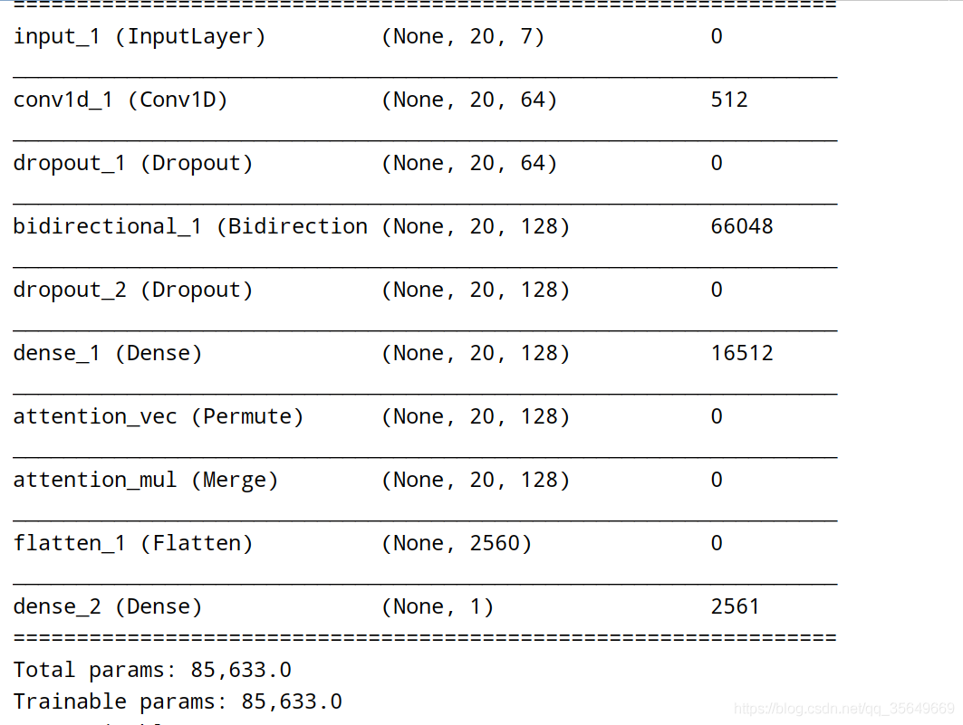
The structure of the model is shown in the figure ,

To make predictions

Before we choose 80% Data for training , after 20% Data to predict , Predict the next moment pollution data .

data = pd.read_csv("./pollution.csv")
# notes : For the convenience of demonstration, it is not used wnd_dir, In fact, it can be converted into a number sequence through code 
data = data.drop(['wnd_dir'], axis = 1)
data = data.iloc[:int(0.8*data.shape[0]),:]
print(" The length is ",data.shape[0])

The evaluation index

The selected evaluation index is RMSE,MAE,MAPE

import  numpy as np
from  sklearn import  metrics

def GetRMSE(y_hat,y_test):
    sum = np.sqrt(metrics.mean_squared_error(y_test, y_hat))
    return  sum

def GetMAE(y_hat,y_test):
    sum = metrics.mean_absolute_error(y_test, y_hat)
    return  sum

def GetMAPE(y_hat,y_test):
    sum = np.mean(np.abs((y_hat - y_test) / y_test)) * 100
    return sum

Predicted results :

because y_test promising 0 The elements of , So we delete it and ask MAPE
The results are as follows :
RMSE by 26.184022062997542
MAE by 13.882745963353731
MAPE by 22.928112428670353

summary

In this blog , Provides a complete set of modeling - forecast - Evaluation method , Is readily available
It realizes a method of long-term trend memory
There is still room for improvement in prediction accuracy ( There are many reasons , The author uses this method on a large number of data to predict the effect is very good )

notes :
Environmental Science : Keras 2.2 & Tensorflow 1.13.1
The code has been uploaded to my github
If you feel good, you can go github Point a star ( For the sake of renting servers to run experiments )
Reference resources :
LSTNet_keras
LSTNet