Flow based depth generation model

1 introduction

  up to now , Two generation models $\mathrm{G}\mathrm{A}\mathrm{N}$ and $\mathrm{V}\mathrm{A}\mathrm{E}$ It can not be accurately obtained from real data $\mathbf{x}\in \mathcal{D}$ Learning probability distribution in middle school $p(\mathbf{x})$. Take the generation model of implicit variables as an example , Calculating integral $p(\mathbf{x})=\int p(\mathbf{x}|\mathbf{z})d\mathbf{z}$ when , You need to traverse all the implicit variables $\mathbf{z}$ This is very difficult , And impractical . be based on $\mathrm{F}\mathrm{l}\mathrm{o}\mathrm{w}$ The generation model in regularized flow （ Regularized flow is a very powerful tool for estimating probability distribution ） This problem can be better solved with help . A probability distribution $p(\mathbf{x})$ A good estimate can accomplish many tasks , For example, data generation , Estimate the probability of predicting future events , Data sample enhancement, etc .

2 Types of generated models

  Currently, there are three types of generation models , The difference is based on $\mathrm{G}\mathrm{A}\mathrm{N}$ The generation model of , be based on $\mathrm{V}\mathrm{A}\mathrm{E}$ A generation model based on $\mathrm{F}\mathrm{l}\mathrm{o}\mathrm{w}$ The generation model of ：

• Generative antagonistic network （GAN）： GAN It is composed of two neural networks , They are generator and discriminator . The purpose of the generator is to get rid of noise $\mathbf{z}$ Learning to generate real data samples ${\mathbf{x}}^{\prime }$, The purpose of the discriminator is to distinguish the real samples $\mathbf{x}$ And generated samples ${\mathbf{x}}^{\prime }$. During the training , Two networks are playing one $\min \text{-}\max$ To promote and improve each other in the game .
• Variational automatic encoder （VAE）： GAN It is also composed of two neural networks , Encoder and decoder respectively . The encoder is a sample of data $\mathbf{x}$ Encode as hidden vector $\mathbf{z}$, The decoder will hide the vector $\mathbf{z}$ Map back to sample data ${\mathbf{x}}^{\prime }$.VAE Is in the lower bound of the maximum variation , Roughly optimize the log likelihood estimation of data .
• be based on $\mathrm{F}\mathrm{l}\mathrm{o}\mathrm{w}$ The generation model of ： One is based on $\mathrm{F}\mathrm{l}\mathrm{o}\mathrm{w}$ The generation model is composed of a series of reversible converters . It can make the model learn the data distribution more accurately $p(\mathbf{x})$, Its loss function is a negative log likelihood function .
  

3 Preliminary knowledge

  In understanding based on $\mathrm{F}\mathrm{l}\mathrm{o}\mathrm{w}$ Before generating the model for , You need to know three key mathematical concepts , They are Jacobian matrix , Determinant and variable substitution theorem .

3.1 Jacobian matrix and determinant

  Given a mapping function $f:{\mathbb{R}}^n\to {\mathbb{R}}^m$, take $n$ Dimensional input vector $\mathbf{x}$ It maps to $m$ The output vector of dimension . Jacobian matrix is a function $f$ About input vectors $\mathbf{x}$ The first partial derivative of all components
$$\mathbf{J}=\left[\begin{array}{ccc}\frac{\partial f_1}{\partial x_1}& \cdots & \frac{\partial f_1}{\partial x_n}\\ ⋮& \ddots & ⋮\\ \frac{\partial f_m}{\partial x_1}& \cdots & \frac{\partial f_m}{\partial x_n}\end{array}\right]$$ The determinant is used to calculate a square matrix , The result is a real valued scalar . The absolute value of the determinant can be considered as “ How much space does the multiplication of a matrix expand or contract ” The measurement . One $n\times n$ Matrix $M$ The determinant of is as follows $$\mathrm{d}\mathrm{e}\mathrm{t}(M)=\mathrm{d}\mathrm{e}\mathrm{t}\left(\left[\begin{array}{cccc}{a}_{11}& a_{12}& \cdots & a_{1n}\\ a_{21}& a_{22}& \cdots & a_{2n}\\ ⋮& ⋮& \ddots & ⋮\\ a_{n1}& a_{n2}& \cdots & a_{nn}\end{array}\right]\right)=\sum _{j_1{j}_2\cdots j_n}(-1{)}^{\tau (j_1{j}_2\cdots j_n)}{a}_{1j_1}{a}_{2j_2}\cdots a_{n{j}_n}$$ Where the subscript under the sum $j_1{j}_2\cdots j_n$ Is a collection $\{1,\cdots ,n\}$ All permutations of , share $n!$ term .$\tau$ It represents the symbol of replacement . Matrix $M$ The value of determinant is $0$ when , Is irreversible , vice versa . The determinant product formula is $$\mathrm{d}\mathrm{e}\mathrm{t}(AB)=\mathrm{d}\mathrm{e}\mathrm{t}(A)\cdot \mathrm{d}\mathrm{e}\mathrm{t}(B)$$

3.2 Variable substitution theorem

  Given a single variable random variable $z$, Its probability distribution is known to be $z\sim \pi (z)$, If you want to use a mapping function $f$ Construct a new random variable $x$, namely $x=f(z)$, among $f$ It's reversible , namely $z=f^{-1}(x)$, Then the probability distribution of the new random variable is derived as follows $$\int p(x)dx=\int \pi (z)dz=1$$$$p(x)=\pi (z)\frac{dz}{dx}=\pi (f^{-1}(x))\frac{d{f}^{-1}}{dx}=\pi (f^{-1}(x))|(f^{-1}{)}^{\prime }(x)|$$ By definition , integral $\int \pi (z)dz$ Is an infinite number of widths $\Delta z$ The sum of infinitesimal rectangles . This location $z$ The height of the rectangle at is a function of density $\pi (z)$ Value . When a variable is replaced , from $z=f^{-1}(x)$ obtain $\frac{\Delta z}{\Delta x}=(f^{-1}(x){)}^{\prime }$ and $\Delta z=(f^{-1}(x){)}^{\prime }$.$|f^{-1}(x){|}^{\prime }$ Represents the ratio between rectangular areas defined in two different variable coordinates . The version of the multivariable is as follows ：
$$\mathbf{z}\sim \pi (\mathbf{z}),\mathbf{x}=f(\mathbf{z}),\mathbf{z}=f^{-1}(\mathbf{x})$$$$p(\mathbf{x})=\pi (\mathbf{z})\cdot \mathrm{d}\mathrm{e}\mathrm{t}\left(\frac{d\mathbf{z}}{d\mathbf{x}}\right)=\pi (f^{-1}(\mathbf{x}))\cdot \mathrm{d}\mathrm{e}\mathrm{t}\left(\frac{d{f}^{-1}}{d\mathbf{x}}\right)$$ among $\mathrm{d}\mathrm{e}\mathrm{t}\left(\frac{\partial f}{\partial \mathbf{z}}\right)$ Is the determinant of Jacobian matrix .

4 Standardized flow

  Good density estimation of probability distribution has direct application in many machine learning problems , But this is very difficult . for example , Because we need to run back propagation in the deep learning model , So the probability distribution of the embedded variable （ A posteriori $p(\mathbf{z}|\mathbf{x})$） The prediction is simple enough , Derivatives can be calculated easily and efficiently . This is why Gaussian distribution is often used in implicit variable generation models , Although most real-world distributions are much more complex than Gaussian distributions . Standardized flow models can be used for better 、 More powerful distribution approximation . The normalized flow transforms a simple distribution into a complex distribution by applying a series of reversible transformation functions . Through a series of transformations , Replace new variables repeatedly according to the variable replacement theorem , Finally, the probability distribution of the final target variable is obtained .

As shown in the figure above , The corresponding formula is
$$\begin{array}{rl}{\mathbf{z}}_{i-1}& \sim p_{i-1}({\mathbf{z}}_{i-1})\\ {\mathbf{z}}_i& =f_i({\mathbf{z}}_{i-1}),{\mathbf{z}}_{i-1}=f_i^{-1}({\mathbf{z}}_i)\\ p_i({\mathbf{z}}_i)& =p_i(f_i^{-1}({\mathbf{z}}_i))\cdot \mathrm{d}\mathrm{e}\mathrm{t}\frac{d{f}_i^{-1}}{d{\mathbf{z}}_i}\end{array}$$ According to the above formula, we can deduce the probability distribution $p_i({\mathbf{z}}_i)$ Expressed as $$\begin{array}{rl}{p}_i({\mathbf{z}}_i)& =p_{i-1}(f_i^{-1}({\mathbf{z}}_i))\cdot \mathrm{d}\mathrm{e}\mathrm{t}\left(\frac{d{f}_i^{-1}}{d{\mathbf{z}}_i}\right)\\ & =p_{i-1}({\mathbf{z}}_{i-1})\cdot \mathrm{d}\mathrm{e}\mathrm{t}{\left(\frac{d{f}_i}{d{\mathbf{z}}_{i-1}}\right)}^{-1}\\ & =p_{i-1}({\mathbf{z}}_{i-1})\cdot {\left[\mathrm{d}\mathrm{e}\mathrm{t}\left(\frac{d{f}_i}{d{\mathbf{z}}_{i-1}}\right)\right]}^{-1}\\ \log p_i({\mathbf{z}}_i)& =\log p_{i-1}({\mathbf{z}}_{i-1})-\log \mathrm{d}\mathrm{e}\mathrm{t}\left(\frac{d{f}_i}{d{\mathbf{z}}_{i-1}}\right)\end{array}$$ The inverse function theorem is used in the derivation of the above formula , That is, if $y=f(x)$ And $x=f^{-1}(y)$, Then there are
$$\frac{d{f}^{-1}(y)}{dy}=\frac{dx}{dy}={\left(\frac{dy}{dx}\right)}^{-1}={\left(\frac{df(x)}{dx}\right)}^{-1}$$ The inverse function theorem of Jacobian matrix is ： The determinant of the inverse of a reversible matrix is the reciprocal of the determinant of the matrix , namely $\mathrm{d}\mathrm{e}\mathrm{t}(M^{-1})=(\mathrm{d}\mathrm{e}\mathrm{t}(M){)}^{-1}$, because $\mathrm{d}\mathrm{e}\mathrm{t}(M)\cdot \mathrm{d}\mathrm{e}\mathrm{t}(M^{-1})=\mathrm{d}\mathrm{e}\mathrm{t}(M\cdot M^{-1})=\mathrm{d}\mathrm{e}\mathrm{t}(I)=1$. Given such a series of probability density functions , We know the relationship between each pair of continuous variables . So you can output $\mathbf{x}$ Until we trace back to the initial distribution ${\mathbf{z}}_0$.$$\begin{array}{rl}\mathbf{x}={\mathbf{z}}_k& =f_K\circ f_{K-1}\circ \cdots f_1({\mathbf{z}}_0)\\ \log p(\mathbf{x})=\log {\pi }_K({\mathbf{z}}_K)& =\log {\pi }_{K-1}({\mathbf{z}}_{K-1})-\log \mathrm{d}\mathrm{e}\mathrm{t}\left(\frac{d{f}_K}{d{\mathbf{z}}_{K-1}}\right)\\ & =\log {\pi }_{K-2}({\mathbf{z}}_{K-2})-\log \mathrm{d}\mathrm{e}\mathrm{t}\left(\frac{d{f}_{K-1}}{d{\mathbf{z}}_{K-2}}\right)-\log \mathrm{d}\mathrm{e}\mathrm{t}\left(\frac{d{f}_K}{d{\mathbf{z}}_{K-1}}\right)\\ & =\cdots \\ & =\log {\pi }_0({\mathbf{z}}_0)-\sum _{i=1}^K\log \det \left(\frac{d{f}_i}{d{\mathbf{z}}_{i-1}}\right)\end{array}$$ A random variable ${\mathbf{z}}_i=f_i({\mathbf{z}}_{i-1})$ The path through is a stream , Continuous distribution ${\pi }_i$ The whole chain formed is called a standardized flow . According to the calculation requirements of the equation , The transformation function should satisfy two properties , It is easy to calculate the determinant of function reversibility and Jacobian matrix respectively .

5 Standardized flow

  It becomes easier to calculate the exact log likelihood of input data through standardized flow , The training loss function of the flow based generation model is the negative log likelihood on the training data set $$\mathcal{L}(\mathcal{D})=-\frac{1}{|\mathcal{D}|}\sum _{\mathbf{x}\in \mathcal{D}}\log p(\mathbf{x})$$

5.1 RealNVP

 RealNVP The model realizes the standardization flow by superimposing the reversible bijective transformation function sequence . In every double shot $f:\mathbf{x}\to y$ in , The input dimension is divided into two parts ：

• $d$ Dimensions remain the same ;
• The first $d+1$ Dimension to $D$ dimension , Affine transformation （“ Zoom and pan ”）, The zoom and translation parameters are functions of the first dimension .$$\begin{array}{rl}{\mathbf{y}}_{1:d}& ={\mathbf{x}}_{1:d}\\ {\mathbf{y}}_{d+1:D}& ={\mathbf{x}}_{d+1:D}\odot \exp (s({\mathbf{x}}_{1:d}))+t({\mathbf{x}}_{1:d})\end{array}$$ among $s(\cdot )$ and $t(\cdot )$ Is the zoom and translation function , The mappings are ${\mathbb{R}}^d\to {\mathbb{R}}^{D-d}$,$\odot$ The product by element represented by the operator .

For the condition of normalized flow 1 Is a function invertible in RealNVP It is very easy to implement in the model , The specific functions are as follows $$\{\begin{array}{rl}{\mathbf{y}}_{1:d}& ={\mathbf{x}}_{1:d}\\ {\mathbf{y}}_{d+1:D}& ={\mathbf{x}}_{d+1:D}\odot \exp (s({\mathbf{x}}_{1:d}))+t({\mathbf{x}}_{1:d})\end{array}*\{\begin{array}{rl}{\mathbf{x}}_{1:d}& ={\mathbf{y}}_{1:d}\\ {\mathbf{x}}_{d+1:D}& =({\mathbf{y}}_{d+1:D}-t({\mathbf{y}}_{1:d}))\odot \exp (-s({\mathbf{y}}_{1:d}))\end{array}$$
For normalized flow conditions 2 The middle Jacobian determinant is easy to calculate in RealNVP The model can also be implemented , Its Jacobian matrix is a lower triangular matrix , The specific matrix is as follows $$\mathbf{J}=\left[\begin{array}{cc}{\mathbb{I}}_d& 0_{d\times (D-d)}\\ \frac{\partial {\mathbf{y}}_{d+1:D}}{\partial {\mathbf{x}}_{1:d}}& \mathrm{d}\mathrm{i}\mathrm{a}\mathrm{g}(\exp (s({\mathbf{x}}_{1:d})))\end{array}\right]$$ therefore , Determinant is simply product of the terms on diagonal .$$\mathrm{d}\mathrm{e}\mathrm{t}(\mathbf{J})=\prod _{j=1}^{D-d}\exp (s({\mathbf{x}}_{1:d}){)}_j=\exp \left(\sum _{j=1}^{D-d}s({\mathbf{x}}_{1:d}{)}_j\right)$$ up to now , The affine coupling layer looks very suitable for building standardized flows . What's better is , Because of the calculation $f^{-1}$ There is no need to calculate $s$ or $t$ The inverse of , And the calculation of Jacobian determinant does not involve calculation $s$ or $t$ Jacobian matrix of , So these functions can be arbitrarily complex , Both can be modeled using deep neural networks . In an affine coupling layer , Some dimensions （ passageway ） remain unchanged . To ensure that all inputs have a chance to be changed , The model reverses the order in each layer , So that different module components remain unchanged . In this alternating pattern , Keeping the same set of cells in one transformation layer is always modified in the next transformation layer . Batch standardization helps train models with very deep coupling layer stacks . Besides ,RealNVP Can work in a multi-scale Architecture , Build more efficient models for large inputs . Multi-scale architecture will be a number of “ sampling ” Operation applied to generic affine layer , Including spatial checkerboard pattern masking 、 Compression operation and channel masking .
 NICE The model is RealNVP The previous work of ,NICE The transformation in is an affine coupling layer without scale terms , It is called additive coupling layer $$\{\begin{array}{rl}{\mathbf{y}}_{1:d}& ={\mathbf{x}}_{1:d}\\ {\mathbf{y}}_{d+1:D}& ={\mathbf{x}}_{d+1:D}+m({\mathbf{x}}_{1:d})\end{array}*\{\begin{array}{rl}{\mathbf{x}}_{1:d}& ={\mathbf{y}}_{1:d}\\ {\mathbf{x}}_{d+1:D}& ={\mathbf{y}}_{d+1:D}-m({\mathbf{y}}_{1:d})\end{array}$$

5.2 Glow

 $\mathrm{G}\mathrm{l}\mathrm{o}\mathrm{w}$ The model extends the previous reversible generation model $\mathrm{N}\mathrm{I}\mathrm{C}\mathrm{E}$ and $\mathrm{R}\mathrm{e}\mathrm{a}\mathrm{l}\mathrm{N}\mathrm{V}\mathrm{P}$, And by reversible $1\times 1$ Convolution replaces the reverse permutation operation on channel sorting to simplify the architecture .$\mathrm{G}\mathrm{l}\mathrm{o}\mathrm{w}$ A step in a process in contains three sub steps ：

• Activate normalization ： It performs affine transformations using the scale and bias parameters of each channel , Similar to batch normalization , But it is applicable to the batch size of $1$. The parameters are trainable , But initialized , Therefore, the small batch data has a mean value of... After activation and normalization $0$ And the standard deviation is $1$.
• reversible $1\times 1$ Convolution ： stay $\mathrm{R}\mathrm{e}\mathrm{a}\mathrm{l}\mathrm{N}\mathrm{V}\mathrm{P}$ Between the layers of the flow , The order of channels is the opposite , Therefore, all data dimensions have the opportunity to be changed . Having the same number of input and output channels $1\times 1$ Convolution is a generalization of any channel permutation . Suppose there is an input tensor dimension called tensor $\mathbf{h}\in {\mathbb{R}}^{h\times w\times c}$ Reversible $1\times 1$ Convolution , Its weight matrix is $\mathbf{W}\in {\mathbb{R}}^{c\times c}$. The output is a $h\times w\times c$ Tensor , Write it down as $f=\mathrm{c}\mathrm{o}\mathrm{n}\mathrm{v}2\mathrm{d}(\mathbf{h};\mathbf{W})$. In order to apply the variable substitution theorem , You need to compute the Jacobian determinant $\left|\mathrm{d}\mathrm{e}\mathrm{t}\left(\frac{\partial f}{\partial \mathbf{h}}\right)\right|$.$\mathbf{h}$ Every element in ${\mathbf{x}}_{ij}(i=1,\cdots ,h,j=1,\cdots ,2)$ It's a $c$ Vector of the number of channels , Each element is multiplied by the weight matrix to obtain the corresponding element in the output matrix ${\mathbf{y}}_{ij}$. The derivative of each element is $\frac{\partial {\mathbf{x}}_{ij}\mathbf{W}}{\partial {\mathbf{x}}_{ij}}=\mathbf{W}$, And there are altogether $h\times w$ Elements ：
  $$\log \det \left(\frac{\partial \mathrm{c}\mathrm{o}\mathrm{n}\mathrm{v}2\mathrm{d}(\mathbf{h};\mathbf{W})}{\partial \mathbf{h}}\right)=\log (|\mathrm{d}\mathrm{e}\mathrm{t}(\mathbf{W}){|}^{h\cdot w})=h\cdot w\cdot \log |\det (\mathbf{W})|$$ reversible $1\times 1$ Convolution depends on inverse matrix $\mathbf{W}$. Because the weight matrix is relatively small , Therefore, the calculation of matrix determinant and inverse is still in a controllable range .
• Affine coupling layer ：$\mathrm{G}\mathrm{l}\mathrm{o}\mathrm{w}$ The structure design of affine coupling layer and $\mathrm{R}\mathrm{e}\mathrm{a}\mathrm{l}\mathrm{N}\mathrm{V}\mathrm{P}$ The affine coupling layer is the same .

6 The model of autoregressive flow

  An autoregressive constraint is a constraint on a sequence of data $\mathbf{x}=[x_1,\cdots ,x_D]$ Modeling method ： Each output depends only on data observed in the past , Without relying on future data . let me put it another way , Probability of observation $x_i$ Is dependent on sequence data $x_1,\cdots ,x_{i-1}$, The product of these conditional probabilities provides the probability of observing the complete sequence ：$$p(\mathbf{x})=\prod _{i=1}^{D}p(x_i|x_1,\cdots ,x_{i-1})=\prod _{i=1}^{D}p(x_i|x_{1:i-1})$$

6.1 MADE

 $\mathrm{M}\mathrm{A}\mathrm{D}\mathrm{E}$ Is a specially designed architecture , Autoregressive attributes can be effectively performed in the auto encoder . When using an automatic encoder to predict conditional probabilities ,$\mathrm{M}\mathrm{A}\mathrm{D}\mathrm{E}$ It is not an input that provides different viewing window times to the automatic encoder , Instead, the contribution of some hidden units is eliminated by multiplying the binary mask matrix , So that each input dimension is only reconstructed from a given previous dimension for one-time propagation . Given a $L$ A hidden layer fully connected neural network , Its weight matrix is ${\mathbf{W}}^1,\cdots {\mathbf{W}}^L$, And an output layer weight matrix $\mathbf{V}$, Each dimension of the output has ${\hat{x}}_i=p(x_i|x_{1:i-1})$, When there is no mask matrix , The process of neural network forward propagation is as follows ：$$\begin{array}{rl}{\mathbf{h}}^0& =\mathbf{x}\\ {\mathbf{h}}^l& ={\mathrm{a}\mathrm{c}\mathrm{t}\mathrm{i}\mathrm{v}\mathrm{a}\mathrm{t}\mathrm{i}\mathrm{o}\mathrm{n}}^l({\mathbf{W}}^l{\mathbf{h}}^{l-1}+{\mathbf{b}}^l)\\ \hat{\mathbf{x}}& =\sigma (\mathbf{V}{\mathbf{h}}^L+\mathbf{c})\end{array}$$ To zero some connections between layers , Each weight matrix can be simply multiplied by a binary mask matrix by its elements . Each hidden node is assigned a random “ Concatenate integers ”, Be situated between $1$ and $D-1$ Between ; The first $k$ In the middle of the layer $l$ The assigned value of cells is expressed as $m_k^l$. The binary mask matrix is determined by comparing the values of two nodes in the two layers element by element , Then there are $$\begin{array}{rl}{\mathbf{h}}^l& ={\mathrm{a}\mathrm{c}\mathrm{t}\mathrm{i}\mathrm{v}\mathrm{a}\mathrm{t}\mathrm{i}\mathrm{o}\mathrm{n}}^l(({\mathbf{W}}^l\odot {\mathbf{M}}^{{\mathbf{W}}^l}){\mathbf{h}}^{l-1}+{\mathbf{b}}^l)\\ \hat{\mathbf{x}}& =\sigma ((\mathbf{V}\odot {\mathbf{M}}^{\mathbf{V}}){\mathbf{h}}^L+\mathbf{c})\\ M_{k^{\prime },k}^{{\mathbf{W}}^l}& =1_{m_{k^{\prime }}^l\ge m_k^{l-1}}=\{\begin{array}{ll}1,& \mathrm{i}\mathrm{f}{m}_{k^{\prime }}^l\ge m_k^{l-1}\\ 0,& \mathrm{o}\mathrm{t}\mathrm{h}\mathrm{e}\mathrm{r}\mathrm{w}\mathrm{i}\mathrm{s}\mathrm{e}\end{array}\\ M_{d,k}^{\mathbf{V}}& =1_{d\ge m_k^L}=\{\begin{array}{ll}1,& \mathrm{i}\mathrm{f}d>m_k^L\\ 0,& \mathrm{o}\mathrm{t}\mathrm{h}\mathrm{e}\mathrm{r}\mathrm{w}\mathrm{i}\mathrm{s}\mathrm{e}\end{array}\end{array}$$ An example is shown in the figure below , A cell in the current layer can only be connected to other cells with the same or smaller random number in the previous layer , And this type of dependency can be easily propagated to the output layer through the network . Once random numbers are assigned to all cells and layers , The order in which dimensions are entered is fixed , And relative to it, it produces a conditional probability . To ensure that all hidden cells are connected to the input and output layers through some paths , sampling $m_k^l$ Equal to or greater than the smallest connected integer in the previous layer ${\min }_{k^{\prime }}{m}_{k^{\prime }}^{l-1}$

6.2 WaveNet

 $\mathrm{W}\mathrm{a}\mathrm{v}\mathrm{e}\mathrm{N}\mathrm{e}\mathrm{t}$ It consists of a stack of causal convolutions , This is a convolution operation designed to respect sorting ： Prediction at a time stamp can only consume data observed in the past , Not dependent on the future .$\mathrm{W}\mathrm{a}\mathrm{v}\mathrm{e}\mathrm{N}\mathrm{e}\mathrm{t}$ The causal convolution in just moves the output multiple timestamps into the future , So that the output is aligned with the last input element . One of the disadvantages of convolution layer is that the size of perception field is very limited . The output can hardly depend on the input hundreds or thousands of time steps ago , This may be a key requirement for long sequence modeling . therefore ,$\mathrm{W}\mathrm{a}\mathrm{v}\mathrm{e}\mathrm{N}\mathrm{e}\mathrm{t}$ Using extended convolution , The kernel is applied to the uniformly distributed sample subset in the larger perceptual field of input .$\mathrm{W}\mathrm{a}\mathrm{v}\mathrm{e}\mathrm{N}\mathrm{e}\mathrm{t}$ The gated activation unit is used as the nonlinear layer , Because it is found to be better than in modeling one-dimensional audio data $\mathrm{R}\mathrm{e}\mathrm{L}\mathrm{U}$ Work better , Apply residual connection after gating activation , The formula is as follows $$\mathbf{z}=\mathrm{t}\mathrm{a}\mathrm{n}\mathrm{h}({\mathbf{W}}_{f,k}\otimes \mathbf{x})\odot \sigma ({\mathbf{W}}_{g,k}\otimes \mathbf{x})$$ among ${\mathbf{W}}_{f,k}$ and ${\mathbf{W}}_{g,k}$ They are the first $k$ Layer convolution filter and gate weight matrix , Both are learnable .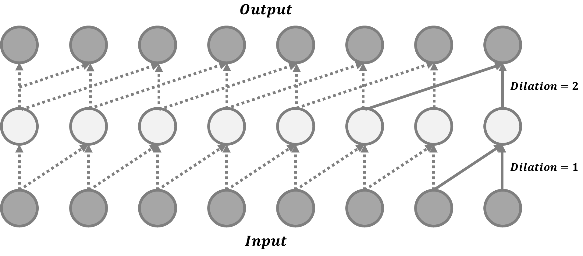

6.3 MAF

 $\mathrm{M}\mathrm{A}\mathrm{F}$ Is a standardized flow , The transformation layer is constructed as an autoregressive neural network . $\mathrm{M}\mathrm{A}\mathrm{F}$ It's the same as the following $\mathrm{I}\mathrm{A}\mathrm{F}$ Very similar . Given two random variables $\mathbf{z}\sim \pi (\mathbf{z})$ and $\mathbf{x}\sim p(\mathbf{x})$, And the probability density function $\pi (\mathbf{z})$ It is known that ,$\mathrm{M}\mathrm{A}\mathrm{F}$ Aims at learning $p(\mathbf{x})$.$\mathrm{M}\mathrm{A}\mathrm{F}$ Generate each $x_i$ In the dimension of the past ${\mathbf{x}}_{1:i-1}$ On condition that . To be exact , The conditional probability is $\mathbf{z}$ The affine transformation of , Where the scale and shift terms are $\mathbf{x}$ Function of the observation part of . Data generation , Will produce a new $\mathbf{x}$, The formula is as follows $$x_i\sim p(x_i|{\mathbf{x}}_{1:i-1})=z_i\odot {\sigma }_i({\mathbf{x}}_{1:i-1})+{\mu }_i({\mathbf{x}}_{1:i-1})$$ Given $\mathbf{x}$ when , The density is estimated to be $$p(\mathbf{x})=\prod _{i=1}^{D}p(x_i|{\mathbf{x}}_{1:i-1})$$ The method advantage of this framework is that the generation process is sequential , So the design speed is very slow . Density estimation only needs to use $\mathrm{M}\mathrm{A}\mathrm{D}\mathrm{E}$ And so on . The inverse of the transformation function is very simple , Jacobian determinant is also easy to calculate .

6.4 IAF

  And $\mathrm{M}\mathrm{A}\mathrm{F}$ similar , Inverse autoregressive flow $\mathrm{I}\mathrm{A}\mathrm{F}$ The conditional probability of the target variable is also modeled as an autoregressive model , But with reverse flow , Thus, a very effective sampling process is realized .$\mathrm{M}\mathrm{A}\mathrm{F}$ The affine transformation in is ：$$z_i=\frac{x_i-{\mu }_i({\mathbf{x}}_{1:i-1})}{{\sigma }_i({\mathbf{x}}_{1:i-1})}=-\frac{{\mu }_i({\mathbf{x}}_{1:i-1})}{{\sigma }_i({\mathbf{x}}_{1:i-1})}+x_i\odot \frac{1}{{\sigma }_i({\mathbf{x}}_{1:i-1})}$$ If you make
$$\begin{array}{rl}& \tilde{\mathbf{x}}=\mathbf{z},\tilde{p}(\cdot )=\pi (\cdot ),\tilde{\mathbf{x}}\sim \tilde{p}(\tilde{\mathbf{x}})\\ & \tilde{\mathbf{x}}=\mathbf{x},\tilde{\pi }(\cdot )=p(\cdot ),\tilde{\mathbf{z}}\sim \tilde{\pi }(\tilde{\mathbf{z}})\\ & {\tilde{\mu }}_i({\tilde{\mathbf{z}}}_{1:i-1})={\tilde{\mu }}_i({\mathbf{x}}_{1:i-1})=-\frac{{\mu }_i({\mathbf{x}}_{1:i-1})}{{\sigma }_i({\mathbf{x}}_{1:i-1})}\\ & \tilde{\sigma }({\tilde{\mathbf{z}}}_{1:i-1})=\tilde{\sigma }({\mathbf{x}}_{1:i-1})=\frac{1}{{\sigma }_i({\mathbf{x}}_{1:i-1})}\end{array}$$ Then there are $${\tilde{x}}_i\sim p({\tilde{x}}_i|{\tilde{\mathbf{z}}}_{1:i})={\tilde{z}}_i\odot {\tilde{\sigma }}_i({\tilde{\mathbf{z}}}_{1:i-1})+{\tilde{\mu }}_i({\tilde{\mathbf{z}}}_{1:i-1}),\mathrm{w}\mathrm{h}\mathrm{e}\mathrm{r}\mathrm{e}\tilde{\mathbf{z}}\sim \tilde{\pi }(\tilde{\mathbf{z}})$$ As shown in the figure below ,$\mathrm{I}\mathrm{A}\mathrm{F}$ Intend to estimate known $\tilde{\pi }(\tilde{\mathbf{z}})$ Given by $\tilde{\mathbf{x}}$ The probability density function of . Countercurrent is also an autoregressive affine transformation , And $\mathrm{M}\mathrm{A}\mathrm{F}$ identical , But the scale and shift terms are known distributions $\tilde{\pi }(\tilde{\mathbf{z}})$ The autoregressive function of the observed variable in .

Single element ${\tilde{x}}_i$ The calculations of are not interdependent , So they are easy to parallelize . It is known that $\tilde{\mathbf{x}}$ The efficiency of density estimation is not high , Because it must be restored in sequence ${\tilde{z}}_i$ Value , That is to say ${\tilde{z}}_i=({\tilde{x}}_i-{\tilde{\mu }}_i({\tilde{\mathbf{z}}}_{1:i-1}))/{\tilde{\sigma }}_i({\mathbf{z}}_{1:i-1})$, So the total needs $D$ Secondary estimate .